ipyrad command line tutorial - Part I
This is the first part of the full tutorial for the command line interface (CLI) for ipyrad. In this tutorial we’ll walk through the entire assembly and analysis process. This is meant as a broad introduction to familiarize users with the general workflow, and some of the parameters and terminology. We will continue with assembly and analysis of the Anolis dataset of Prates et al. 2016, which we fetched during the previous QC analysis step. This data was generated with the GBS protocol and sequenced single-end (SE), but the core concepts will apply to assembly of other data types (ddRAD and paired-end (PE)).
If you are new to RADseq analyses, this tutorial will provide a simple overview of how to execute ipyrad, what the data files look like, how to check that your analysis is working, and what the final output formats will be.
Each grey cell in this tutorial indicates a command line interaction.
Lines starting with $ indicate a command that should be executed
in a terminal connected to the USP cluster, for example by copying and
pasting the text into your terminal. Elements in code cells surrounded
by angle brackets (e.g.
## Example Code Cell.
## Create an empty file in my home directory called `watdo.txt`
$ touch ~/watdo.txt

## Print "wat" to the screen
$ echo "wat"
wat
Overview of Assembly Steps
Very roughly speaking, ipyrad exists to transform raw data coming off the sequencing instrument into output files that you can use for downstream analysis.
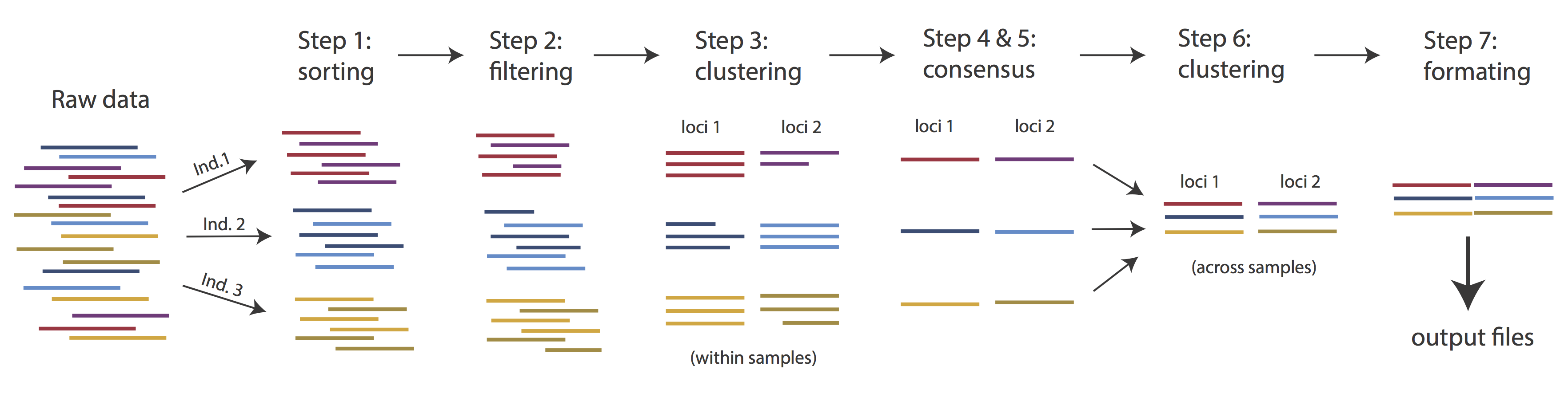
The basic steps of this process are as follows:
- Step 1 - Demultiplex/Load Raw Data
- Step 2 - Trim and Quality Control
- Step 3 - Cluster within Samples
- Step 4 - Calculate Error Rate and Heterozygosity
- Step 5 - Call consensus sequences
- Step 6 - Cluster across Samples
- Step 7 - Apply filters and write output formats
Note on files in the project directory: Assembling rad-seq type sequence data requires a lot of different steps, and these steps generate a lot of intermediary files. ipyrad organizes these files into directories, and it prepends the name of your assembly to each directory with data that belongs to it. One result of this is that you can have multiple assemblies of the same raw data with different parameter settings and you don’t have to manage all the files yourself! (See Branching assemblies for more info). Another result is that you should not rename or move any of the directories inside your project directory, unless you know what you’re doing or you don’t mind if your assembly breaks.
Getting Started
If you haven’t already installed ipyrad go here first: installation
Working with the cluster
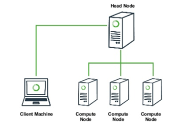
A typical high performance computing (HPC) cluster architecture looks somewhat like this, just with many many more “compute nodes”. The “head node” (or login node) is normally the only system that you will interact with. If you want to run a big job on the cluster, you will connect to the head node (with ssh), and will submit a job to the ‘work queue’. In this job you specify how many cores you want to run on, how much RAM you want, and how much time you think it’ll take. Then the work queue looks at your job and at all the other jobs in the queue and figures out when is the fairest time to start your job running. This can be almost immediately, or your job might sit in the queue for hours or days, if the system is very busy. Either way, you will rarely actually “see” your job run because you normally aren’t given access to the compute nodes directly.
This is usually okay, because usually if you want to run a “big” job, this means you want to run tons of small, quick tasks, or one or a few really really huges and slow tasks, and you kind of don’t care what’s happening, so long as they finish at some point. For us, for the benefit of exposing and monitoring the processes for the tutorial, having jobs locked away in the work queue is inconvenient. Fortunately, many HPC systems provide an “interactive” mode, which allows you to run certain limited tasks inside a terminal directly on one of the compute nodes.
Therefore, we will run all our assembly and analysis on the USP cluster
inside an “interactive” job. This will allow us to run our proccesses on
compute nodes, but still be able to remain at the command line so
we can easily monitor progress. If you do not still have an active
ssh window on the cluster, begin by re-establishing the connection
through puTTY (Windows) or
ssh (Mac/Linux):
$ ssh <username>@lem.ib.usp.br
Submitting an interactive job to the cluster
Now we will submit an interactive job with relatively modest resource requests. Remember, you can see default and maximum resource allocations for all cluster queues here.
## -q proto         - Submit a job to the 'prototyping' queue
## -l nodes=1:ppn=2 - Request 2 processes on the target compute node
## -l mem=64        - Request 64Gb of main memory
## -I               - Use 'interactive' mode (get a terminal on the compute node)

$ qsub -q proto -l nodes=1:ppn=2 -l mem=64gb -I
qsub: waiting for job 24816.darwin to start
qsub: job 24816.darwin ready
Depending on cluster usage the job submission script can take more
or less time to, but the USP cluster is normally quite fast, so it this
request shouldn’t take more than a few moments. Once you see the
qsub: job XXXX.darwin ready message this indicates that your
interactive job request was successful and your terminal is now
running on a compute node.
Inspecting running cluster processes
At any time you can ask the cluster for the status of your jobs with the
qstat command. For a simple qstat call, the most interesting column
is marked S (meaning “status”). The most common values for this field
are:
- R - Job is running
- Q - job is queued (boo!)
- C - Job is completed (yay!)
## Check the status of my running job on the 'proto' Queue
$ qstat
Job ID                    Name             User            Time Use S Queue
------------------------- ---------------- --------------- -------- - -----
24817.darwin              STDIN            isaac           00:00:00 R proto

## Ask more detailed information about job status with the `-r` flag
$ qstat -r

darwin:
                                                                                  Req'd       Req'd       Elap
Job ID                  Username    Queue    Jobname          SessID  NDS   TSK   Memory      Time    S   Time
----------------------- ----------- -------- ---------------- ------ ----- ------ --------- --------- - ---------
24817.darwin            isaac       proto    STDIN             38014     1      2      64gb  04:00:00 R  00:00:07
ipyrad help
To better understand how to use ipyrad, let’s take a look at the help argument. We will use some of the ipyrad arguments in this tutorial (for example: -n, -p, -s, -c, -r). But, the complete list of optional arguments and their explanation goes below.
$ ipyrad --help
usage: ipyrad [-h] [-v] [-r] [-f] [-q] [-d] [-n new] [-p params]
              [-b [branch [branch ...]]] [-m [merge [merge ...]]] [-s steps]
              [-c cores] [-t threading] [--MPI] [--preview]
              [--ipcluster [ipcluster]] [--download [download [download ...]]]

optional arguments:
  -h, --help            show this help message and exit
  -v, --version         show program's version number and exit
  -r, --results         show results summary for Assembly in params.txt and
                        exit
  -f, --force           force overwrite of existing data
  -q, --quiet           do not print to stderror or stdout.
  -d, --debug           print lots more info to ipyrad_log.txt.
  -n new                create new file 'params-{new}.txt' in current
                        directory
  -p params             path to params file for Assembly:
                        params-{assembly_name}.txt
  -b [branch [branch ...]]
                        create a new branch of the Assembly as
                        params-{branch}.txt
  -m [merge [merge ...]]
                        merge all assemblies provided into a new assembly
  -s steps              Set of assembly steps to perform, e.g., -s 123
                        (Default=None)
  -c cores              number of CPU cores to use (Default=0=All)
  -t threading          tune threading of binaries (Default=2)
  --MPI                 connect to parallel CPUs across multiple nodes
  --preview             run ipyrad in preview mode. Subset the input file so
                        it'll runquickly so you can verify everything is
                        working
  --ipcluster [ipcluster]
                        connect to ipcluster profile (default: 'default')
  --download [download [download ...]]
                        download fastq files by accession (e.g., SRP or SRR)

  * Example command-line usage:
    ipyrad -n data                       ## create new file called params-data.txt
    ipyrad -p params-data.txt            ## run ipyrad with settings in params file
    ipyrad -p params-data.txt -s 123     ## run only steps 1-3 of assembly.
    ipyrad -p params-data.txt -s 3 -f    ## run step 3, overwrite existing data.

  * HPC parallelization across 32 cores
    ipyrad -p params-data.txt -s 3 -c 32 --MPI

  * Print results summary
    ipyrad -p params-data.txt -r

  * Branch/Merging Assemblies
    ipyrad -p params-data.txt -b newdata
    ipyrad -m newdata params-1.txt params-2.txt [params-3.txt, ...]

  * Subsample taxa during branching
    ipyrad -p params-data.txt -b newdata taxaKeepList.txt

  * Download sequence data from SRA into directory 'sra-fastqs/'
    ipyrad --download SRP021469 sra-fastqs/

  * Documentation: http://ipyrad.readthedocs.io
Create a new parameters file
ipyrad uses a text file to hold all the parameters for a given assembly.
Start by creating a new parameters file with the -n flag. This flag
requires you to pass in a name for your assembly. In the example we use
anolis but the name can be anything at all. Once you start
analysing your own data you might call your parameters file something
more informative, like the name of your organism and some details on the settings.
$ cd ~/ipyrad-workshop
$ ipyrad -n anolis
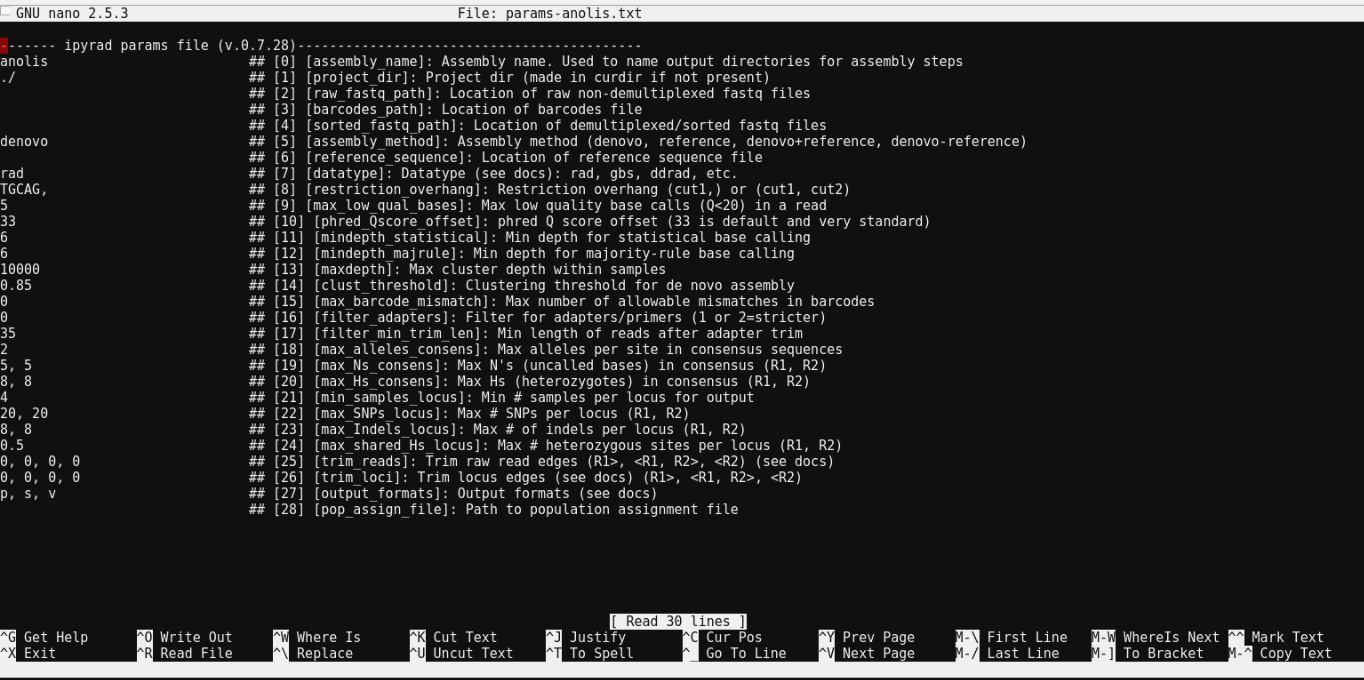
This will create a file in the current directory called
params-anolis.txt. The params file lists on each line one
parameter followed by a ## mark, then the name of the parameter, and
then a short description of its purpose. Lets take a look at it.
$ cat params-anolis.txt
------- ipyrad params file (v.0.7.28)-------------------------------------------
anolis                         ## [0] [assembly_name]: Assembly name. Used to name output directories for assembly steps
./                             ## [1] [project_dir]: Project dir (made in curdir if not present)
                               ## [2] [raw_fastq_path]: Location of raw non-demultiplexed fastq files
                               ## [3] [barcodes_path]: Location of barcodes file
                               ## [4] [sorted_fastq_path]: Location of demultiplexed/sorted fastq files
denovo                         ## [5] [assembly_method]: Assembly method (denovo, reference, denovo+reference, denovo-reference)
                               ## [6] [reference_sequence]: Location of reference sequence file
rad                            ## [7] [datatype]: Datatype (see docs): rad, gbs, ddrad, etc.
TGCAG,                         ## [8] [restriction_overhang]: Restriction overhang (cut1,) or (cut1, cut2)
5                              ## [9] [max_low_qual_bases]: Max low quality base calls (Q<20) in a read
33                             ## [10] [phred_Qscore_offset]: phred Q score offset (33 is default and very standard)
6                              ## [11] [mindepth_statistical]: Min depth for statistical base calling
6                              ## [12] [mindepth_majrule]: Min depth for majority-rule base calling
10000                          ## [13] [maxdepth]: Max cluster depth within samples
0.85                           ## [14] [clust_threshold]: Clustering threshold for de novo assembly
0                              ## [15] [max_barcode_mismatch]: Max number of allowable mismatches in barcodes
0                              ## [16] [filter_adapters]: Filter for adapters/primers (1 or 2=stricter)
35                             ## [17] [filter_min_trim_len]: Min length of reads after adapter trim
2                              ## [18] [max_alleles_consens]: Max alleles per site in consensus sequences
5, 5                           ## [19] [max_Ns_consens]: Max N's (uncalled bases) in consensus (R1, R2)
8, 8                           ## [20] [max_Hs_consens]: Max Hs (heterozygotes) in consensus (R1, R2)
4                              ## [21] [min_samples_locus]: Min # samples per locus for output
20, 20                         ## [22] [max_SNPs_locus]: Max # SNPs per locus (R1, R2)
8, 8                           ## [23] [max_Indels_locus]: Max # of indels per locus (R1, R2)
0.5                            ## [24] [max_shared_Hs_locus]: Max # heterozygous sites per locus (R1, R2)
0, 0, 0, 0                     ## [25] [trim_reads]: Trim raw read edges (R1>, <R1, R2>, <R2) (see docs)
0, 0, 0, 0                     ## [26] [trim_loci]: Trim locus edges (see docs) (R1>, <R1, R2>, <R2)
p, s, v                        ## [27] [output_formats]: Output formats (see docs)
                               ## [28] [pop_assign_file]: Path to population assignment file
In general the defaults are sensible, and we won’t mess with them for now, but there are a few parameters we must change: the path to the raw data, the dataype, and the restriction overhang sequence.
We will use the nano text editor to modify params-anolis.txt and change
these parameters:
$ nano params-anolis.txt
Nano is a command line editor, so you’ll need to use only the arrow keys on the keyboard for navigating around the file. Nano accepts a few special keyboard commands for doing things other than modifying text, and it lists these on the bottom of the frame.
We need to specify that the raw data files are in the raws directory, that
our data used the gbs library prep protocol, and that the overhang left by
our restriction enzyme is TGCAT (reflecting the use of EcoT22I by Prates
et al. 2016). Change the following values in the params file to match these:
./raws/*.gz                    ## [4] [sorted_fastq_path]: Location of demultiplexed/sorted fastq files
gbs                            ## [7] [datatype]: Datatype (see docs): rad, gbs, ddrad, etc.
TGCAT,                         ## [8] [restriction_overhang]: Restriction overhang (cut1,) or (cut1, cut2)
After you change these parameters you may save and exit nano by typing CTRL+o (to write Output), and then CTRL+x (to eXit the program).
Note: The
CTRL+xnotation indicates that you should hold down the control key (which is often styled ‘ctrl’ on the keyboard) and then push ‘x’.
Once we start running the analysis ipyrad will create several new
directories to hold the output of each step for this assembly. By
default the new directories are created in the project_dir
directory and use the prefix specified by the assembly_name parameter.
Because we use ./ for the project_dir for this tutorial, all these
intermediate directories will be of the form: /home/<username/ipyrad-workshop/anolis_*.
Note: Again, the
./notation indicates the current working directory. You can always view the current working directory with thepwdcommand (print working directory).
Input data format
Before we get started let’s take a look at what the raw data looks like.
Your input data will be in fastQ format, usually ending in .fq,
.fastq, .fq.gz, or .fastq.gz. The file/s may be compressed with
gzip so that they have a .gz ending, but they do not need to be. When loading
pre-demultiplexed data (as we are with the Anolis data) the location
of raw sample files should be entered on line 3 of the params file. Below are the
first three reads of one of the Anolis files.
## For your personal edification here is what this is doing:
## gunzip -c: Tells gzip to unzip the file and write the contents to the screen
## head -n 12: Grabs the first 12 lines of the fastq file. Fastq files
## have 4 lines per read, so the value of `-n` should be a multiple of 4

$ gunzip -c ./raws/punc_IBSPCRIB0361_R1_.fastq.gz | head -n 12

@D00656:123:C6P86ANXX:8:2201:3857:34366 1:Y:0:8
TGCATGTTTATTGTCTATGTAAAAGGAAAAGCCATGCTATCAGAGATTGGCCTGGGGGGGGGGGGCAAATACATGAAAAAGGGAAAGGCAAAATG
+
;=11>111>1;EDGB1;=DG1=>1:EGG1>:>11?CE1<>1<1<E1>ED1111:00CC..86DG>....//8CDD/8C/....68..6.:8....
@D00656:123:C6P86ANXX:8:2201:5076:34300 1:N:0:8
TGCATATGAACCCCAACCTCCCCATCACATTCCACCATAGCAATCAGTTTCCTCTCTTCCTTCTTCTTGACCTCTCCACCTCAAAGGCAACTGCA
+
@;BFGEBCC11=/;/E/CFGGGG1ECCE:EFDFCGGGGGGG11EFGGGGGCGG:B0=F0=FF0=F:FG:FDG00:;@DGGDG@0:E0=C>DGCF0
@D00656:123:C6P86ANXX:8:2201:5042:34398 1:N:0:8
TGCATTCAAAGGGAGAAGAGTACAGAAACCAAGCACATATTTGAAAAATGCAAGATCGGAAGAGCGGTTCAGCAGGAATGCCGAGACCGATCTCG
+
GGGGGGGCGGGGGGGGGGGGGEGGGFGGGGGGEGGGGGGGGGGGGGFGGGEGGGGGGGGGGGGGGGGGGGGGGGGGGGEGGGGGGGGG@@DGGGG
Each read is composed of four lines. The first is the name of the read (its location on the plate). The second line contains the sequence data. The third line is unused. And the fourth line is the quality scores for the base calls. The FASTQ wikipedia page has a good figure depicting the logic behind how quality scores are encoded.
The Anolis data are 96bp single-end reads prepared as GBS. The first five bases (TGCAT) form the restriction site overhang. All following bases make up the sequence data.
Step 1: Loading the raw data files
With reads already demultiplexed to samples, step 1 simply scans through the raw data, verifies the input format, and counts reads per sample. It doesn’t create any new directories or modify the raw files in any way.
Note on step 1: More commonly, rather than returning demultiplexed samples as we have here, sequencing facilities will give you one giant .gz file that contains all the sequences from your run. This situation only slightly modifies step 1, and does not modify further steps, so we will refer you to the full ipyrad tutorial for guidance in this case.
Now lets run step 1! For the Anolis data this will take <1 minute.
Special Note: In interactive mode on the USP cluster please be aware of always specifying the number of cores with the
-cflag. If you do not specify the number of cores ipyrad assumes you want all of them, and this will make your run very fast, but it might aggravate the cluster usage for everyone else.
## -p    the params file we wish to use
## -s    the step to run
## -c    the number of cores to allocate   <-- Important!
$ ipyrad -p params-anolis.txt -s 1 -c 2

 -------------------------------------------------------------
  ipyrad [v.0.7.28]
  Interactive assembly and analysis of RAD-seq data
 -------------------------------------------------------------
  New Assembly: anolis
  establishing parallel connection:
  host compute node: [2 cores] on darwin

  Step 1: Loading sorted fastq data to Samples
  [####################] 100%  loading reads         | 0:00:04
  10 fastq files loaded to 10 Samples.
In-depth operations of running an ipyrad step
Any time ipyrad is invoked it performs a few housekeeping operations:
- Load the assembly object - Since this is our first time running any steps we need to initialize our assembly.
- Start the parallel cluster - ipyrad uses a parallelization library called ipyparallel. Every time we start a step we fire up the parallel clients. This makes your assemblies go smokin’ fast.
- Do the work - Actually perform the work of the requested step(s) (in this case loading in sample reads).
- Save, clean up, and exit - Save the state of the assembly, and spin down the ipyparallel cluster.
As a convenience ipyrad internally tracks the state of all your steps in your
current assembly, so at any time you can ask for results by invoking the -r flag.
## -r fetches informative results from currently executed steps
$ ipyrad -p params-anolis.txt -r

Summary stats of Assembly anolis
------------------------------------------------
                   state  reads_raw
punc_IBSPCRIB0361      1     250000
punc_ICST764           1     250000
punc_JFT773            1     250000
punc_MTR05978          1     250000
punc_MTR17744          1     250000
punc_MTR21545          1     250000
punc_MTR34414          1     250000
punc_MTRX1468          1     250000
punc_MTRX1478          1     250000
punc_MUFAL9635         1     250000


Full stats files
------------------------------------------------
step 1: ./anolis_s1_demultiplex_stats.txt
step 2: None
step 3: None
step 4: None
step 5: None
step 6: None
step 7: None
If you want to get even more info ipyrad tracks all kinds of wacky stats and saves them to a file inside the directories it creates for each step. For instance to see full stats for step 1 (the wackyness of the step 1 stats at this point isn’t very interesting, but we’ll see stats for later steps are more verbose):
$ cat anolis_s1_demultiplex_stats.txt

                   reads_raw
punc_IBSPCRIB0361     250000
punc_ICST764          250000
punc_JFT773           250000
punc_MTR05978         250000
punc_MTR17744         250000
punc_MTR21545         250000
punc_MTR34414         250000
punc_MTRX1468         250000
punc_MTRX1478         250000
punc_MUFAL9635        250000
Step 2: Filter reads
This step filters reads based on quality scores and maximum number of uncalled bases, and can be used to detect Illumina adapters in your reads, which is sometimes a problem under couple different library prep scenarios. Recalling from our exploration of the data with FastQC we have some problem with adapters, and a little noise toward the 3’ end. To account for this we will trim reads to 75bp and set adapter filtering to be quite aggressive.
Note: Trimming to 75bp seems a bit aggressive too, and based on the FastQC results you probably would not want to do this with if these were your real data. However, it will speed up the analysis considerably. Here, we are just trimming the reads for the sake of this workshop.
Edit your params file again with nano:
nano params-anolis.txt
and change the following two parameter settings:
2                               ## [16] [filter_adapters]: Filter for adapters/primers (1 or 2=stricter)
0, 75, 0, 0                     ## [25] [trim_reads]: Trim raw read edges (R1>, <R1, R2>, <R2) (see docs)
Note: Saving and quitting from
nano:CTRL+othenCTRL+x
$ ipyrad -p params-anolis.txt -s 2 -c 2

 -------------------------------------------------------------
  ipyrad [v.0.7.28]
  Interactive assembly and analysis of RAD-seq data
 -------------------------------------------------------------
  loading Assembly: anolis
  from saved path: ~/ipyrad-workshop/anolis.json
  establishing parallel connection:
  host compute node: [2 cores] on darwin

  Step 2: Filtering reads
  [####################] 100%  processing reads      | 0:01:02
The filtered files are written to a new directory called anolis_edits. Again,
you can look at the results output by this step and also some handy stats tracked
for this assembly.
## View the output of step 2
$ cat anolis_edits/s2_rawedit_stats.txt
                   reads_raw  trim_adapter_bp_read1  trim_quality_bp_read1  reads_filtered_by_Ns  reads_filtered_by_minlen  reads_passed_filter
punc_IBSPCRIB0361     250000                 108761                 160210                    66                     12415               237519
punc_ICST764          250000                 107320                 178463                    68                     13117               236815
punc_JFT773           250000                 110684                 190803                    46                      9852               240102
punc_MTR05978         250000                 102932                 144773                    54                     12242               237704
punc_MTR17744         250000                 103394                 211363                    55                      9549               240396
punc_MTR21545         250000                 119191                 161709                    63                     21972               227965
punc_MTR34414         250000                 109207                 193401                    54                     16372               233574
punc_MTRX1468         250000                 119746                 134069                    45                     19052               230903
punc_MTRX1478         250000                 116009                 184189                    53                     16549               233398
punc_MUFAL9635        250000                 114492                 182877                    61                     18071               231868
## Get current stats including # raw reads and # reads after filtering.
$ ipyrad -p params-anolis.txt -r
You might also take a closer look at the filtered reads:
$ gunzip -c anolis_edits/punc_IBSPCRIB0361.trimmed_R1_.fastq.gz | head -n 12

@D00656:123:C6P86ANXX:8:2201:3857:34366 1:Y:0:8
TGCATGTTTATTGTCTATGTAAAAGGAAAAGCCATGCTATCAGAGATTGGCCTGGGGGGGGGGGGCAAATACATG
+
;=11>111>1;EDGB1;=DG1=>1:EGG1>:>11?CE1<>1<1<E1>ED1111:00CC..86DG>....//8CDD
@D00656:123:C6P86ANXX:8:2201:5076:34300 1:N:0:8
TGCATATGAACCCCAACCTCCCCATCACATTCCACCATAGCAATCAGTTTCCTCTCTTCCTTCTTCTTGACCTCT
+
@;BFGEBCC11=/;/E/CFGGGG1ECCE:EFDFCGGGGGGG11EFGGGGGCGG:B0=F0=FF0=F:FG:FDG00:
@D00656:123:C6P86ANXX:8:2201:5042:34398 1:N:0:8
TGCATTCAAAGGGAGAAGAGTACAGAAACCAAGCACATATTTGAAAAATGCA
+
GGGGGGGCGGGGGGGGGGGGGEGGGFGGGGGGEGGGGGGGGGGGGGFGGGEG
This is actually really cool, because we can already see the results of both of our applied parameters. All reads have been trimmed to 75bp, and the third read had adapter contamination removed (you can tell because it’s shorter than 75bp). As an exercise you can go back up to the section where we looked at the raw data initially and see if you can identify the adapter sequence in this read.
Step 3: clustering within-samples
Step 3 de-replicates and then clusters reads within each sample by the
set clustering threshold and then writes the clusters to new files in a
directory called anolis_clust_0.85. Intuitively we are trying to
identify all the reads that map to the same locus within each sample.
The clustering threshold specifies the minimum percentage of sequence
similarity below which we will consider two reads to have come from
different loci.
The true name of this output directory will be dictated by the value you
set for the clust_threshold parameter in the params file.
You can see the default value is 0.85, so our default directory is named accordingly. This value dictates the percentage of sequence similarity that reads must have in order to be considered reads at the same locus. You’ll more than likely want to experiment with this value, but 0.85 is a reliable default, balancing over-splitting of loci vs over-lumping. Don’t mess with this until you feel comfortable with the overall workflow, and also until you’ve learned about Branching assemblies.
It’s also possible to incorporate information from a reference genome to improve clustering at this this step, if such a resources is available for your organism (or one that is relatively closely related). We will not cover reference based assemblies in this workshop, but you can refer to the ipyrad documentation for more information.
Note on performance: Steps 3 and 6 generally take considerably longer than any of the steps, due to the resource intensive clustering and alignment phases. These can take on the order of 10-100x as long as the next longest running step.
Now lets run step 3:
$ ipyrad -p params-anolis.txt -s 3 -c 2

 -------------------------------------------------------------
  ipyrad [v.0.7.28]
  Interactive assembly and analysis of RAD-seq data
 -------------------------------------------------------------
  loading Assembly: anolis
  from saved path: ~/ipyrad-workshop/anolis.json
  establishing parallel connection:
  host compute node: [2 cores] on darwin

  Step 3: Clustering/Mapping reads
  [####################] 100%  dereplicating         | 0:00:11
  [####################] 100%  clustering            | 0:19:35
  [####################] 100%  building clusters     | 0:00:06
  [####################] 100%  chunking              | 0:00:01
  [####################] 100%  aligning              | 0:14:27
  [####################] 100%  concatenating         | 0:00:04```
In-depth operations of step 3:
- dereplicating - Merge all identical reads
- clustering - Find reads matching by sequence similarity threshold
- building clusters - Group similar reads into clusters
- chunking - Subsample cluster files to improve performance of alignment step
- aligning - Align all clusters
- concatenating - Gather chunked clusters into one full file of aligned clusters
Again we can examine the results. The stats output tells you how many clusters were found (‘clusters_total’), and the number of clusters that pass the mindepth thresholds (‘clusters_hidepth’). We’ll go into more detail about mindepth settings in some of the advanced tutorials but for now all you need to know is that by default step 3 will filter out clusters that only have a handful of reads on the assumption that these are probably all mostly due to sequencing error.
$ ipyrad -p params-anolis.txt -r

Summary stats of Assembly anolis
------------------------------------------------
                   state  reads_raw  reads_passed_filter  clusters_total  clusters_hidepth
punc_IBSPCRIB0361      3     250000               237519           56312              4223
punc_ICST764           3     250000               236815           60626              4302
punc_JFT773            3     250000               240102           61304              5214
punc_MTR05978          3     250000               237704           61615              4709
punc_MTR17744          3     250000               240396           62422              5170
punc_MTR21545          3     250000               227965           55845              3614
punc_MTR34414          3     250000               233574           61242              4278
punc_MTRX1468          3     250000               230903           54411              3988
punc_MTRX1478          3     250000               233398           57299              4155
punc_MUFAL9635         3     250000               231868           59249              3866
Again, the final output of step 3 is dereplicated, clustered files for
each sample in ./anolis_clust_0.85/. You can get a feel for what
this looks like by examining a portion of one of the files.
## Same as above, `gunzip -c` unzips and prints to the screen and
## `head -n 28` means just show me the first 28 lines.
$ gunzip -c anolis_clust_0.85/punc_IBSPCRIB0361.clustS.gz | head -n 28

000e3bb624e3bd7e91b47238b7314dc6;size=4;*
TGCATATCACAAGAGAAGAAAGCCACTAATTAAGGGGAAAAGAAAAGCCTCTGATATAGCTCCGATATATCATGC-
75e462e101383cca3db0c02fca80b37a;size=2;-
-GCATATCACAAGAGAAGAAAGCCACTAATTAAGGGGAAAAGAAAAGCCTCTGATATAGCTCCGATATATCATGCA
//
//
0011c57e1e3c03e4a71516bd51c623da;size=1;*
TGCATGAAATAGATACAACTGAGCACATTTGCTTTGTTTCCAGAGAGTGCAACAAGAGTTTGGAGAATATAAATG
eef50f7e4849ed4761f1fd38b08d0e12;size=1;+
TGCATGAAATAGATACTACTGAGCACATTTGCTTTGTTTCCAGAGATTGCATCAAGAGTTTGGAGAATATAAATG
7f089b34522da8288b0e6ff7db8ffc6c;size=1;+
TGCATGAAATAGATACAACTGAGCACATTTGCTTTGTTTCCAGAGATTGCAACAAGAGTTTGGAGAATATAAATG
//
//
001236a2310c39a3a16d96c4c6c48df1;size=4;*
TGCATCTCTTTGGGCTGTTGCTTGGTGGCACACCATGCTGCTTTCTCCTCACTTTTTCTCTCTTTTCCTGAGACT------------------------------
4644056dca0546a270ba897b018624b4;size=2;-
------------------------------CACCATGCTGCTTTCTCCTCACTTTTTCTCTCTTTTCCTGAGACTGAGCCAGGGACAGCGGCTGAGGAGGATGCA
5412b772ec0429af178caf6040d2af30;size=1;+
TGCATTTCTTTGGGCTGTTGCTTGGTGGCACACCATGCTGCTTTCTCCTCACTTTTTCTCTCTTTTCCTGAGACT------------------------------
//
//
0013684f0db0bd454a0a6fd1b160266f;size=1;*
TGCATTGTTCATGAATCGTCCCATTGTATACATTTTACCTGATCTATCTCATTGTATTTTACTCCATGGTTTTCA-------------------------
c26ec07b3e3e77d3167341d100fd2d4e;size=1;-
-------------------------GTATACATTTTACTTGATCTATCTCATTGTATTTTACTCCATGGTTTTCAGTACCTAACAAGCAGCATGTATGCA
55510205b75b441a2c3ce6249f1eb47c;size=1;-
-------------------------GTATACATTTTACCTGATCTATCTTATTGTATTTTACTCCATGGTTTTCAGTACCTAACAAGCAGCATGTATGCA
Reads that are sufficiently similar (based on the above sequence similarity threshold) are grouped together in clusters separated by “//”. For the second and fourth clusters above these are probably homozygous with some sequencing error, but it’s hard to tell. For the first and third clusters, are there truly two alleles (heterozygote)? Is it a homozygote with lots of sequencing errors, or a heterozygote with few reads for one of the alleles?
Thankfully, untangling this mess is what step 4 is all about.