Advanced features of the ipyrad.analysis.pca module
Controlling colors
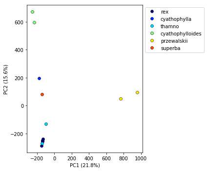
You might notice the default color scheme is unobtrusive, but perhaps not to your liking. There are two ways of modifying the color scheme, one simple and one more complicated, but which gives extremely fine grained control over colors.
Colors for the more complicated method can be specified according to python color conventions. I find this visual page of python color names useful.
## Here's the simple way, just pass in a matplotlib cmap, or even better, the name of a cmap
pca.plot(cmap="jet")
<matplotlib.axes._subplots.AxesSubplot at 0x7fa3d099ac50>
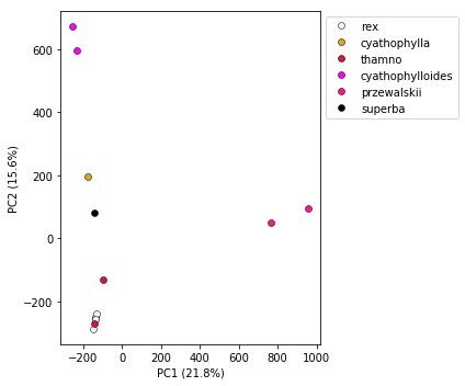
## Here's the harder way that gives you uber control. Pass in a dictionary mapping populations to colors.
my_colors = {
    "rex":"aliceblue",
    "thamno":"crimson",
    "przewalskii":"deeppink",
    "cyathophylloides":"fuchsia",
    "cyathophylla":"goldenrod",
    "superba":"black"
}
pca.plot(cdict=my_colors)
<matplotlib.axes._subplots.AxesSubplot at 0x7fa3d0646b50>
Dealing with missing data
RAD-seq datasets are often characterized by moderate to high levels of missing data. While there may be many thousands or tens of thousands of loci recovered overall, the number of loci that are recovered in all sequenced samples is often quite small. The distribution of depth of coverage per locus is a complicated function of the size of the genome of the focal organism, the restriction enzyme(s) used, the size selection tolerances, and the sequencing effort.
Both model-based (STRUCTURE and the like) and model-free (PCA/sNMF/etc) genetic “clustering” methods are sensitive to missing data. Light to moderate missing data that is distributed randomly among samples is often not enough to seriously impact the results. These are, after all, only exploratory methods. However, if missing data is biased in some way then it can distort the number of inferred populations and/or the relationships among these. For example, if several unrelated samples recover relatively few loci, for whatever reason (mistakes during library prep, failed sequencing, etc), clustering methods may erroniously identify this as true “similarity” with respect to the rest of the samples, and create spurious clusters.
In the end, all these methods must do something with sites that are uncalled in some samples. Some methods adopt a strategy of silently asigning missing sites the “Reference” base. Others, assign missing sites the average base.
There are several ways of dealing with this:
- One method is to simply eliminate all loci with missing data. This can be ok for SNP chip type data, where missingness is very sparse. For RAD-Seq type data, eliminating data for all missing loci often results in a drastic reduction in the size of the final data matrix. Assemblies with thousands of loci can be pared down to only tens or hundreds of loci.
- Another method is to impute missing data. This is rarely done for RAD-Seq type data, comparatively speaking. Or at least it is rarely done intentionally.
- A third method is to downsample using a hypergeometric projection. This is the strategy adopted by dadi in the construction of the SFS (which abhors missing data). It’s a little complicated though, so we’ll only look at the first two strategies.
Inspect the amount of missing data under various conditions
The pca module has various functions for inspecting missing data. The simples is the get_missing_per_sample() function, which does exactly what it says. It displays the number of ungenotyped snps per sample in the final data matrix. Here you can see that since we are using simulated data the amount of missing data is very low, but in real data these numbers will be considerable.
pca.get_missing_per_sample()
1A_0    2
1B_0    2
1C_0    1
1D_0    4
2E_0    0
2F_0    0
2G_0    0
2H_0    1
3I_0    2
3J_0    2
3K_0    1
3L_0    2
dtype: int64
This is useful, but it doesn’t give us a clear direction for how to go about dealing with the missingness. One way to reduce missing data is to reduce the tolerance for samples ungenotyped at a snp. The other way to reduce missing data is to remove samples with very poor sequencing. To this end, the .missingness() function will show a table of number of retained snps for various of these conditions.
pca.missingness()
| Full | 2E_0 | 2F_0 | 2G_0 | 1C_0 | 2H_0 | |
|---|---|---|---|---|---|---|
| 0 | 2547 | 2452 | 2313 | 2093 | 1958 | 1640 |
| 1 | 2553 | 2458 | 2319 | 2098 | 1963 | 1643 |
| 3 | 2554 | 2459 | 2320 | 2099 | 1963 | 1643 |
| 8 | 2555 | 2460 | 2321 | 2099 | 1963 | 1643 |
Here the columns indicate progressive removal of the samples with the fewest number of snps. So “Full” indicates retention of all samples. “2E_0” shows # snps after removing this sample (as it has the most missing data). “2F_0” shows the # snps after removing both this sample & “2E_0”. And so on. You can see as we move from left to right the total number of snps goes down, but also so does the amount of missingness.
Rows indicate thresholds for number of allowed missing samples per snp. The “0” row shows the condition of allowing 0 missing samples, so this is the complete data matrix. The “1” row shows # of snps retained if you allow 1 missing sample. And so on.
Filter by missingness threshold - trim_missing()
The trim_missing() function takes one argument, namely the maximum number of missing samples per snp. Then it removes all sites that don’t pass this threshold.
pca.trim_missing(1)
pca.missingness()
| Full | 1A_0 | 1B_0 | 1C_0 | 2E_0 | 2F_0 | |
|---|---|---|---|---|---|---|
| 0 | 2547 | 2456 | 2282 | 2079 | 1985 | 1845 |
| 1 | 2553 | 2462 | 2286 | 2083 | 1989 | 1849 |
You can see that this also has the effect of reducing the amount of missingness per sample.
pca.get_missing_per_sample()
1A_0    0
1B_0    0
1C_0    0
1D_0    2
2E_0    0
2F_0    0
2G_0    0
2H_0    1
3I_0    1
3J_0    1
3K_0    0
3L_0    1
dtype: int64
NB: This operation is destructive of the data inside the pca object. It doesn’t do anything to your data on file, though, so if you want to rewind you can just reload your vcf file.
## Voila. Back to the full dataset.
pca = ipa.pca(data)
pca.missingness()
| Full | 2E_0 | 2F_0 | 2G_0 | 1C_0 | 2H_0 | |
|---|---|---|---|---|---|---|
| 0 | 2547 | 2452 | 2313 | 2093 | 1958 | 1640 |
| 1 | 2553 | 2458 | 2319 | 2098 | 1963 | 1643 |
| 3 | 2554 | 2459 | 2320 | 2099 | 1963 | 1643 |
| 8 | 2555 | 2460 | 2321 | 2099 | 1963 | 1643 |
Imputing missing genotypes
McVean (2008) recommends filling missing sites with the average genotype of the population, so that’s what we’re doing here. For each population, we determine the average genotype at any site with missing data, and then fill in the missing sites with this average. In this case, if the average “genotype” is “./.”, then this is what gets filled in, so essentially any site missing more than 50% of the data isn’t getting imputed. If two genotypes occur with equal frequency then the average is just picked as the first one.
pca.fill_missing()
pca.missingness()
| Full | 2E_0 | 2F_0 | 2G_0 | 2H_0 | 1C_0 | |
|---|---|---|---|---|---|---|
| 0 | 2553 | 2458 | 2319 | 2099 | 1779 | 1643 |
| 3 | 2554 | 2459 | 2320 | 2100 | 1780 | 1643 |
| 8 | 2555 | 2460 | 2321 | 2100 | 1780 | 1643 |
In comparing this missingness matrix with the previous one, you can see that indeed some snps are being recovered (though not many, again because of the clean simulated data).
You can also examine the effect of imputation on the amount of missingness per sample. You can see it doesn’t have as drastic of an effect as trimming, but it does have some effect, plus you are retaining more data!
pca.get_missing_per_sample()
1A_0    2
1B_0    2
1C_0    1
1D_0    2
2E_0    0
2F_0    0
2G_0    0
2H_0    0
3I_0    1
3J_0    1
3K_0    1
3L_0    1
dtype: int64
Dealing with unequal sampling
Unequal sampling of populations can potentially distort PC analysis (see for example Bradburd et al 2016). Model based ancestry analysis suffers a similar limitation Puechmaille 2016). McVean (2008) recommends downsampling larger populations, but nobody likes throwing away data. Weighted PCA was proposed, but has not been adopted by the community.
{x:len(y) for x, y in pca.pops.items()}
{'cyathophylla': 1,
 'cyathophylloides': 2,
 'przewalskii': 2,
 'rex': 5,
 'superba': 1,
 'thamno': 2}
Dealing with linked snps
prettier_labels = {

    "32082_przewalskii":"przewalskii",
    "33588_przewalskii":"przewalskii",
    "41478_cyathophylloides":"cyathophylloides",
    "41954_cyathophylloides":"cyathophylloides",
    "29154_superba":"superba",
    "30686_cyathophylla":"cyathophylla",
    "33413_thamno":"thamno",
    "30556_thamno":"thamno",
    "35236_rex":"rex",
    "40578_rex":"rex",
    "35855_rex":"rex",
    "39618_rex":"rex",
    "38362_rex":"rex"
}