Setting up the environment and basic quality control
Before we get going with our first RAD-seq assembly, we need to get set up and oriented to our working environment. We make no assumptions about prior experience with cluster environments, so we scaffold the entire participant workshop experience from first principles. More advanced users hopefully will find value in some of the finer details we present.
- Connecting to the Jupyter Hub
- Basic quality control (FastQC)
- Viewing and interpreting FastQC results
Tutorial documentation conventions
Each grey cell in this tutorial indicates a command line interaction. Lines starting with $ indicate a command that should be executed in a terminal, for example by copying and pasting the text into your terminal. All lines in code cells beginning with ## are comments and should not be copied and executed. Elements in code cells surrounded by angle brackets (e.g. <username>) are variables that need to be replaced by the user. All other lines should be interpreted as output from the issued commands.
## Example Code Cell.
## Create an empty file in my home directory called `watdo.txt`
$ touch ~/watdo.txt

## Print "wat" to the screen
$ echo "wat"
wat
Jupyter hub information
Computational resources for the duration of this workshop are being provided by the Eaton lab at Columbia University. We will be using a Jupyter Hub instance running on a 40 core workstation in Deren’s office on the Upper West Side of Manhattan. Using Jupyter Hub allows us to provide pre-configured, isolated computational environments for each participant, skipping over lots of tedious details related to downloading, installing, and configuring software and getting things set up. Jupyter hub allows us to skip straight to the fun stuff! We do provide detailed installation and configuration instructions on the RADCamp site, so that you have some support in getting set up when you return to your home campus.
Connecting to Jupyter Hub
The rest of this tutorial assumes that you have already created a GitHub account. You will need this to gain access to compute resources, so if you haven’t done it yet sign up now.
Once that’s done you can surf your browser to https://jhub.eaton-lab.org/hub/login, and click the big fat orange “Sign in with GitHub” button. This will do a bunch of magic on the backend, and eventually drop you into the browser view of your Jupyter Hub instance.
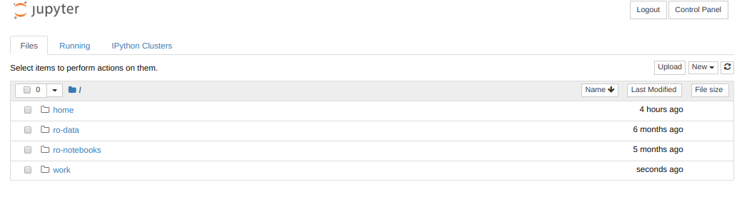
By default everyone will have 4 directories listed in their Jupyter home: home, ro-data, ro-notebooks, and work. Here’s what each of these directories contains:
- home: An empty directory for keeping random stuff. We won’t use this during the workshop.
- ro-data: A
read onlydirectory that houses datasets we’ll use during the workshop. You can read these datasets, but you can’t write to this directory. - ro-notebooks: Example analysis notebooks that you can copy to your working directory to run, modify, and save on your own.
- work: A working directory for creating ipyrad assemblies and analysis output files.
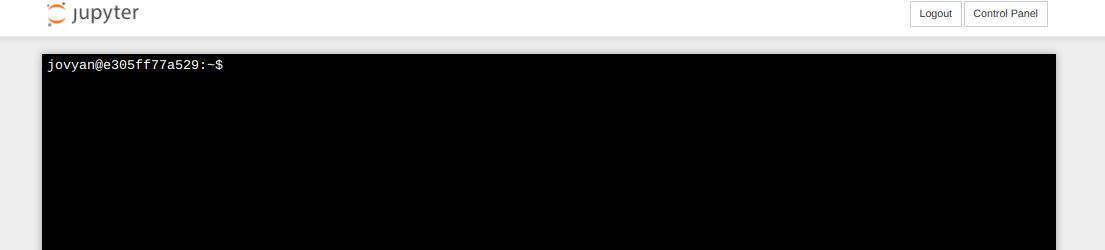
Opening a terminal on the server
From the dashboard ‘Files’ tab choose New->Terminal and you’ll see a new tab pop open with a little black window and a command prompt, like this:
Command line interface (CLI) basics
The CLI provides a way to navigate a file system, move files around, and run commands all inside a little black window. The down side of CLI is that you have to learn many at first seemingly esoteric commands for doing all the things you would normally do with a mouse. However, there are several advantages of CLI: 1) you can use it on servers that don’t have a GUI interface (such as HPC clusters); 2) it’s scriptable, so you can write programs to execute common tasks or run analyses and others can easily reproduce these tasks exactly; 3) it’s often faster and more efficient than click-and-drag GUI interfaces. For now we will start with 4 of the most common and useful commands:
$ pwd
/home/jovyan
pwd stands for “print working directory”, which literally means “where am I now in this filesystem?”. This is a question you should always be aware of when working in a terminal. Just like when you open a file browser window, when you open a new terminal you are located somewhere; the terminal will usually start you out in your “home” directory. Ok, now we know where we are, lets take a look at what’s in this directory:
$ ls
home  ro-data  ro-notebooks  work
ls stands for “list” and you should notice a strong correlation between
the results of ls and the contents of the directories presented by the Jupyter
Hub dashboard. Try to use ls to look inside your home and work directories.
Not Much There. That’s okay, because throughout the workshop we will be
adding files and directories and by the time we’re done, not only will you have
a bunch of experience with RAD-Seq analysis, but you’ll also have a ton of
stuff in your home directory.
Throughout the workshop we will be introducing new commands as the need for them arises. We will pay special attention to highlighting and explaining new commands and giving examples to practice with.
Special Note: Notice that neither of the ‘read-only’ directories are called
ro data, for example. This is very important, as spaces in directory names are known to cause havoc on HPC systems. All linux based operating systems do not recognize file or directory names that include spaces because spaces act as default delimiters between arguments to commands. There are ways around this (for example Mac OS has half-baked “spaces in file names” support) but it will be so much for the better to get in the habit now of never including spaces in file or directory names.
Install ipyrad and various analysis tools
Surprise! We already did this for you. This is one of the strengths of working in a Jupyter Hub environment, that we can curate the Docker image we provide for this workshop (to save time with nitpicky things like installation and configuration). In truth, we rely heavily on the Conda ecosystem for installation of ipyrad and all dependencies. Conda gives us access to an amazing array of analysis tools for both analyzing and manipulating all kinds of data. We provide detailed and explicit ipyrad install instructions on the RADCamp site, which you can explore at your leasure outside this workshop.
Test the version of ipyrad installed inside your compute environment:
$ ipyrad --version
ipyrad 0.8.0.dev0
Examine the raw data
Here we will get hands-on with real data for the first time. We provide three empirical data sets to choose from, and at the workshop we will leave time for exploring this data using some of the ipyrad analysis tools. Each example data set is composed of a dozen or more closely related species or population samples. They are ordered in order of the average divergence among samples. The Anolis data set is a “population-level” data set; the Pedicularis data set is composed of several closely related species and subspecies; and the Finch data set includes several species of finches from two relatively distant clades.
- Prates et al. 2016 (Anolis, single-end GBS).
- Eaton et al. 2013 (Pedicularis, single-end RAD).
- DaCosta and Sorenson 2016 (Finches, single-end ddRAD).
- Simulated datasets
The raw data are located in a special shared folder where we can all access them. Any analyses we run will only read from these files (i.e., they are read-only), not modify them. This is typical of any bioinformatic analysis. We want to develop a set of scripts that start from the unprocessed data and end in new results or statistics. You can use ls to examine the data sets in the shared directory space.
$ ls /home/jovyan/ro-data
ipsimdata  SRP021469  test_outfiles

$ ls /home/joyvan/ro-data/SRP021469
29154_superba_SRR1754715.fastq.gz       33588_przewalskii_SRR1754727.fastq.gz  40578_rex_SRR1754724.fastq.gz
30556_thamno_SRR1754720.fastq.gz        35236_rex_SRR1754731.fastq.gz          41478_cyathophylloides_SRR1754722.fastq.gz
30686_cyathophylla_SRR1754730.fastq.gz  35855_rex_SRR1754726.fastq.gz          41954_cyathophylloides_SRR1754721.fastq.gz
32082_przewalskii_SRR1754729.fastq.gz   38362_rex_SRR1754725.fastq.gz
33413_thamno_SRR1754728.fastq.gz        39618_rex_SRR1754723.fastq.gz
Inspect the data
Then we will use the zcat command to read lines of data from one of the files and we will trim this to print only the first 20 lines by piping the output to the head command. Using a pipe (|) like this passes the output from one command to another and is a common trick in the command line.
Here we have our first look at a fastq formatted file. Each sequenced read is spread over four lines, one of which contains sequence and another the quality scores stored as ASCII characters. The other two lines are used as headers to store information about the read.
$ zcat /home/jovyan/ro-data/SRP021469/29154_superba_SRR1754715.fastq.gz | head -n 20
@29154_superba_SRR1754715.1 GRC13_0027_FC:4:1:12560:1179 length=74
TGCAGGAAGGAGATTTTCGNACGTAGTGNNNNNNNNNNNNNNGCCNTGGATNNANNNGTGTGCGTGAAGAANAN
+29154_superba_SRR1754715.1 GRC13_0027_FC:4:1:12560:1179 length=74
IIIIIIIGIIIIIIFFFFF#EEFE<?################################################
@29154_superba_SRR1754715.2 GRC13_0027_FC:4:1:15976:1183 length=74
TGCAGTTGTAAATACAAATATCCCAAAANNNNGNNNNNNNTNTAATATTTTGNAANNTTGAGGGGTGTGATNTN
+29154_superba_SRR1754715.2 GRC13_0027_FC:4:1:15976:1183 length=74
GGGGHHHHHHHHHHHHHDHGHHHHCAAA##############################################
@29154_superba_SRR1754715.3 GRC13_0027_FC:4:1:19092:1179 length=74
TGCAGGCTCTGACAAAGAANTCGACTGANNNNNNNNNNNNNNCACNGGTTCNNGNNNATGTCAATGTGGTANAN
+29154_superba_SRR1754715.3 GRC13_0027_FC:4:1:19092:1179 length=74
GGGGHHHHBHHBHEB?B@########################################################
@29154_superba_SRR1754715.4 GRC13_0027_FC:4:1:1248:1210 length=74
TGCAGAACTGCTCCCAGAATCTCCAGAAATTGCGAGATTACCCCCAAAATCTCCAGAAATTTCTAGATTACCTC
+29154_superba_SRR1754715.4 GRC13_0027_FC:4:1:1248:1210 length=74
HHHHHDHHHFHHHDHBGHGHHHHHHHGDHE<GGE<D>DGHGGHHHDHHHHHHGHHHHFHHHHHHEHGHHEDEF>
@29154_superba_SRR1754715.5 GRC13_0027_FC:4:1:5242:1226 length=74
TGCAGCAGTCACCAGTCTGGCCCCTACCTCACAAAGTAGCTTGATGGCCGAACCACTCCCAAGGTGAATAGTGC
+29154_superba_SRR1754715.5 GRC13_0027_FC:4:1:5242:1226 length=74
HHHHHHHHHGGGGGHHHGHHHGHGGGGGBHHHBHEE>BGADDDDFHEHFDBGBDCFHBHBB8DD4???::?::?
@29154_superba_SRR1754715.6 GRC13_0027_FC:4:1:12660:1232 length=74
TGCAGGCCCAAAATCAACAATTATGCATAATACAACAAAGTTAATTAATTAATTATATTAAAAAAAGAAAAAGA
+29154_superba_SRR1754715.6 GRC13_0027_FC:4:1:12660:1232 length=74
HHHHHHHHHHHHHHHHHHHHHHHHHHHHGGHHHHFHHHHHHHHHHHHHHHHHHHHHHHHHHHHHHHHHHHHHHH
FastQC for quality control
The first step of any RAD-Seq assembly is to inspect your raw data to estimate overall quality. We began first with a visual inspection above, but of course we can only visually inspect a very tiny proportion of the total data. So instead we use automated approaches to check the quality of our data.
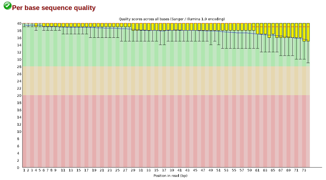
At this stage you can then attempt to improve your dataset by identifying and removing samples with failed sequencing. Another key QC procedure involves inspecting average quality scores per base position and trimming read edges, which is where low quality base-calls tend to accumulate. In this figure, the X-axis shows the position on the read in base-pairs and the Y-axis depicts information about Phred quality score per base for all reads, including median (center red line), IQR (yellow box), and 10%-90% (whiskers). As an example, here is a very clean base sequence quality report for a 75bp RAD-Seq library. These reads have generally high quality across their entire length, with only a slight (barely worth mentioning) dip toward the end of the reads:
In contrast, here is a somewhat typical base sequence quality report for R1 of a 300bp paired-end Illumina run of ezrad data:
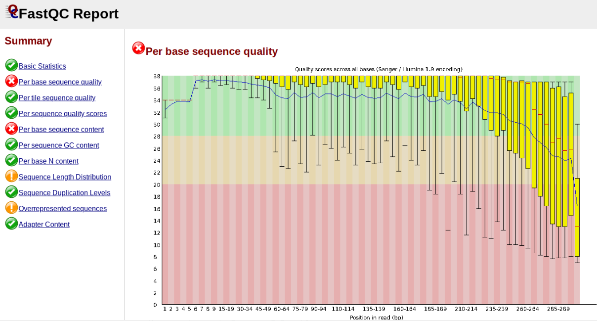
This figure depicts a common artifact of current Illumina chemistry, whereby quality scores per base drop off precipitously toward the ends of reads, with the effect being magnified for read lengths > 150bp. The purpose of using FastQC to examine reads is to determine whether and how much to trim our reads to reduce sequencing error interfering with basecalling. In the above figure, as in most real dataset, we can see there is a tradeoff between throwing out data to increase overall quality by trimming for shorter length, and retaining data to increase value obtained from sequencing with the result of increasing noise toward the ends of reads.
Running FastQC
In the interest of saving time during this short workshop we will only indicate how fastqc is run, and will then focus on interpretation of typical output. More detailed information about actually running fastqc are available elsewhere on the RADCamp site.
To run fastqc on all the pedicularis samples you would execute this command:
$ fastqc -o fastqc-results /home/jovyan/ro-data/SRP021469/*.gz
Note: The -o flag tells fastqc where to write output files. Running this command will create a directory called
fastqc-resultsin your current working directory. Note: The*here is a special command line character that means “Everything that matches this pattern”. So hereSRP021469/*matches everything in the raws directory. Equivalent (though more verbose) statements are:ls SRP021469/*.gz,ls SRP021469/*.fastq.gz. All of these will list all the files in theSRP021469directory. Special Challenge: Can you construct anlscommand using wildcards that only lists samples in theSRP021469directory that include the digit 5 in their sample name?
Inspecting and Interpreting FastQC Output
Now lets spend a moment looking at the results from punc_JFT773_R1__fastqc.html, one of the Anolis samples. Opening up this html file, on the left you’ll see a summary of all the results, which highlights areas FastQC indicates may be worth further examination. We will only look at a few of these.
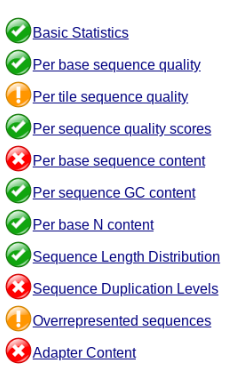
Lets start with Per base sequence quality, because it’s very easy to interpret, and often times with RAD-Seq data results here will be of special importance.
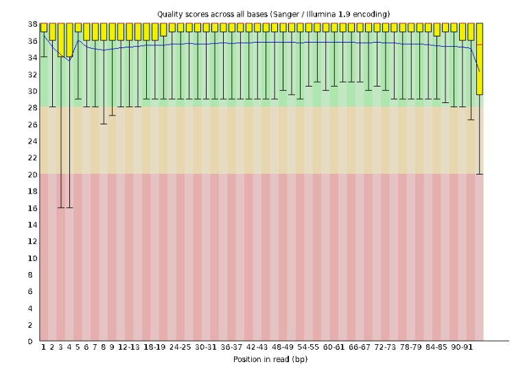
For the Anolis data the sequence quality per base is uniformly quite high, with dips only in the first and last 5 bases (again this is typical for Illumina reads). Based on information from this plot we can see that the Anolis data doesn’t need a whole lot of trimming, which is good.
Now lets look at the Per base sequece content, which FastQC highlights with a scary red X.
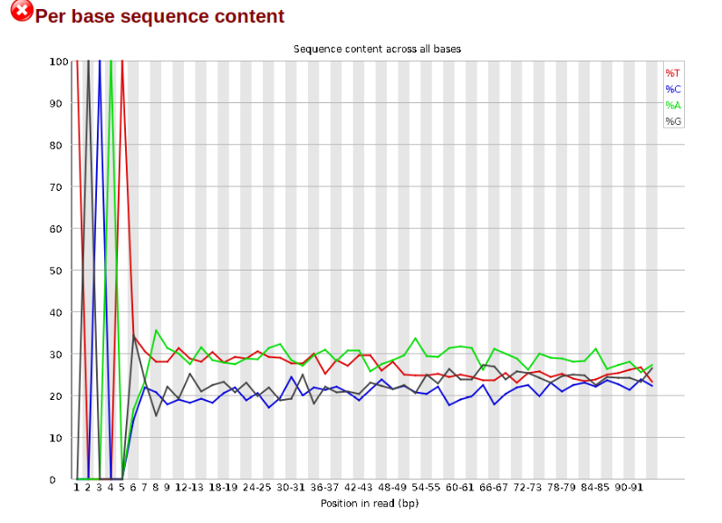
The squiggles indicate base composition per base position averaged across the reads. It looks like the signal FastQC is concerned about here is related to the extreme base composition bias of the first 5 positions. We happen to know this is a result of the restriction enzyme overhang present in all reads (TGCAT in this case for the EcoT22I enzyme used), and so it is in fact of no concern. Now lets look at Adapter Content:
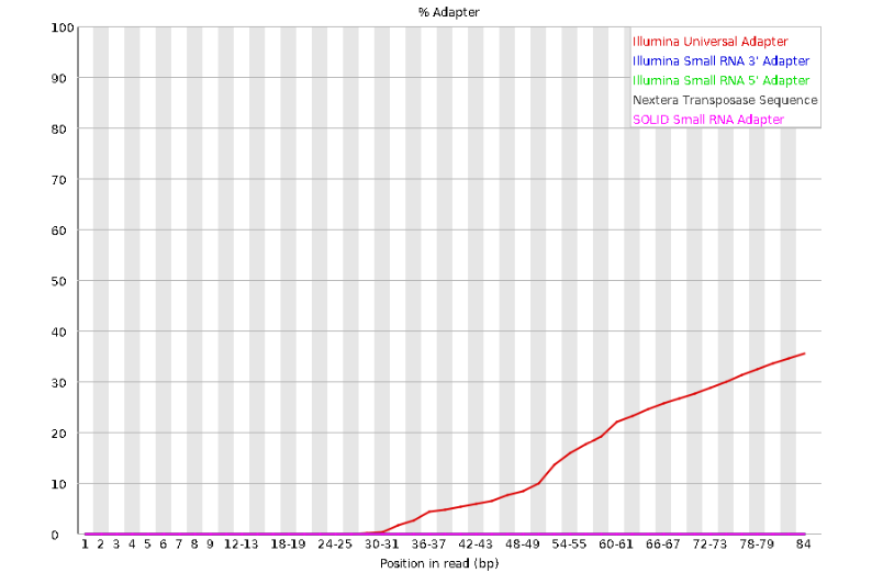
Here we can see adapter contamination increases toward the tail of the reads, approaching 40% of total read content at the very end. The concern here is that if adapters represent some significant fraction of the read pool, then they will be treated as “real” data, and potentially bias downstream analysis. In the Anolis data this looks like it might be a real concern so if we were assembling this dataset we’d want to keep this in mind during step 2 of the ipyrad analysis, and incorporate 3’ read trimming and aggressive adapter filtering.
Other than this, the data look good and we can proceed with the ipyrad analysis.
References
Prates, I., Xue, A. T., Brown, J. L., Alvarado-Serrano, D. F., Rodrigues, M. T., Hickerson, M. J., & Carnaval, A. C. (2016). Inferring responses to climate dynamics from historical demography in neotropical forest lizards. Proceedings of the National Academy of Sciences, 113(29), 7978-7985.