Spatial population genetic analysis: FEEMS

Through methods like PCA and phylogenetic trees, you can gain some insight into how populations cluster together, and which population may be more diverged from each other. But it’s always nice to also look at this in a spatial context, e.g. on a map. FEEMS is a faster version of the statistical method Estimating Effective Migration Surfaces (EEMS), and it is based on the notion of “isolation-by-distance” (IBD). This is the idea that individuals who live near eachother tend to be more similar to individuals who live far apart. EEMS is a good method to visualize deviations from IBD on a map, hereby finding areas where gene flow is less than expected (i.e. barriers; indicated in orange) or areas where gene flow is higher than expected (i.e. increased connectivity; indicated in blue). Below you can see an example for a dataset of lions. The red dots are sampling localities, and you can see some orange shading where EEMS inferred reduced gene flow. For example, in the central African rain forest, the Zambezi valley and the Arabian peninsula.

png

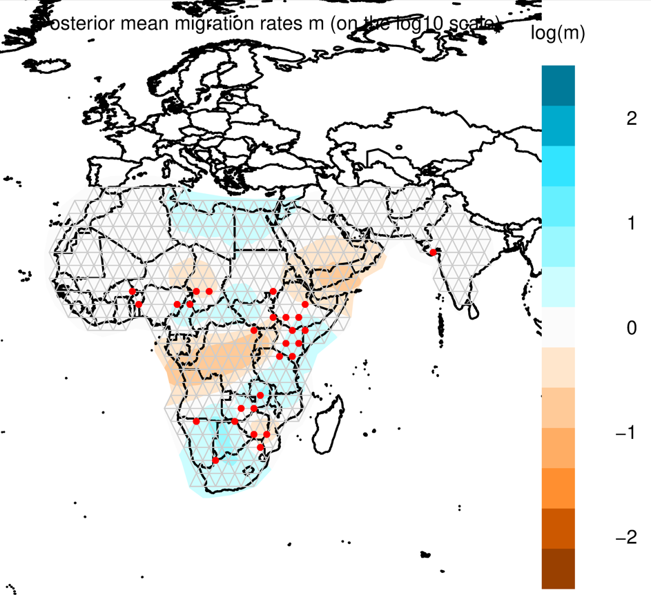
For more information about EEMS, check out Petkova et al (2016), and for FEEMS, check out Marcus et al (2021).

Input data

What is the necessary input data for FEEMS?

genotypes
latlongs (= localities of your samples)
bounding area for plotting
.shp file (global map)

Creating new output files w/o the P. concolor sample

The P. concolor sample was included in the RAxML analysis as an outgroup to root the tree. For this spatial analysis with FEEMS we need to remove this sample because we are interested in gene flow between cheetah populations, and not the outgroup.

We can use the ipyrad branching strategy again to remove this outgroup sample (‘SRR19760949’). Notice here that we are branching from the original assembly with min_samples_locus equal to 4.

(ipyrad) osboxes@osboxes:~/ipyrad-workshop$ ipyrad -p params-cheetah.txt -b no-outgroup - SRR19760949

  loading Assembly: cheetah
  from saved path: ~/ipyrad-workshop/cheetah.json
  dropping 1 samples
  creating a new branch called 'no-outgroup' with 23 Samples
  writing new params file to params-no-outgroup.txt

Now you can run step 7 again to generate the new output files with this sample removed:

(ipyrad) osboxes@osboxes:~/ipyrad-workshop$ ipyrad -p params-no-outgroup.txt -s 7 -c 4

This will create a new set of output files in no-outgroup_outfiles.

FEEMS analyses

Access the FEEMS environment

The FEEMS module requires a substantially different configuration than the other analysis tools in this workshop, so we have installed this software in a separate conda environment with an isolated jupyter notebook server running on a different port. To access this environment open a new browser tab and navigate to:

http://localhost:8801

Create a new notebook for the FEEMS analysis

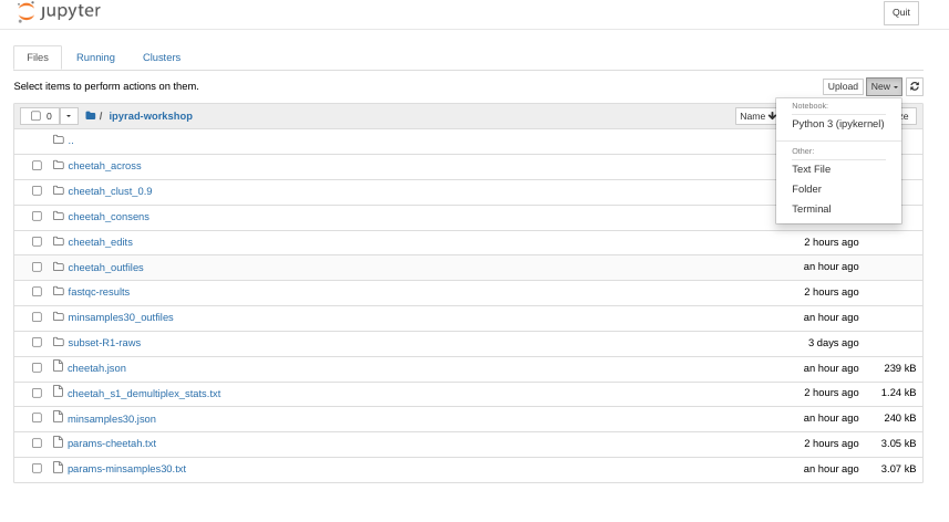
In the jupyter notebook browser interface navigate to your ipyrad-workshop directory and create a “New->Python” Notebook.

png

First things first, rename your new notebook to give it a meaningful name. Choose File->Save Notebook and rename your notebook to “cheetah-FEEMS.ipynb”

Import FEEMS and other necessary modules

The import keyword directs python to load a module into the currently running context. This is very similar to the library() function in R. We begin by importing the ipyrad analysis module. Copy the code below into a notebook cell and click run.

%matplotlib inline

# base
import h5py
import numpy as np
import pandas as pd
from sklearn.impute import SimpleImputer 
# viz 
import matplotlib.pyplot as plt 
import cartopy.crs as ccrs 
# feems 
from feems.utils import prepare_graph_inputs 
from feems import SpatialGraph, Viz 

Import the data and impute missing values

# Path to the input phylip file
data = h5py.File("/home/osboxes/ipyrad-workshop/no-outgroup_outfiles/no-outgroup.snps.hdf5")

raw_genotypes = np.apply_along_axis(np.sum, 2, data["genos"][:])

G = np.where(raw_genotypes <= 2, raw_genotypes, np.nan*raw_genotypes)
imp = SimpleImputer(missing_values=np.nan, strategy="mean") 
genotypes = imp.fit_transform(np.array(G).T) 

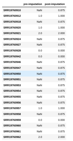
What is ‘imputation’ and why do we need to do it?

locus = 11
print(G[locus])
genotypes[:, locus]

[nan  1. nan  1.  2. nan nan  0.  0. nan nan nan nan nan nan nan nan  1.
 nan  0. nan nan  2.]
array([0.875, 1.   , 0.875, 1.   , 2.   , 0.875, 0.875, 0.   , 0.   ,
       0.875, 0.875, 0.875, 0.875, 0.875, 0.875, 0.875, 0.875, 1.   ,
       0.875, 0.   , 0.875, 0.875, 2.   ])

locus = 11
names = data["snps"].attrs["names"]
pd.DataFrame([G[locus], genotypes[:, locus]], columns=names, index=["pre-imputation", "post-imputation"]).T

png

Fetch the GPS coordinates for the samples and the ‘outer’ points

Typically, you will have information about the sampling localities of your data. FEEMS takes these data as a vector of GPS coördinates, and the file should have the extension .coord. We’ve already prepared this file for you, and you can simply download it.

You also need to provide FEEMS with an outline of the area you want to include in your analysis, and provide this as a file with the extension .outer. You can use the following website to create one, simply by clicking on the map and then copy-pasting the coördinates to a new file.

png

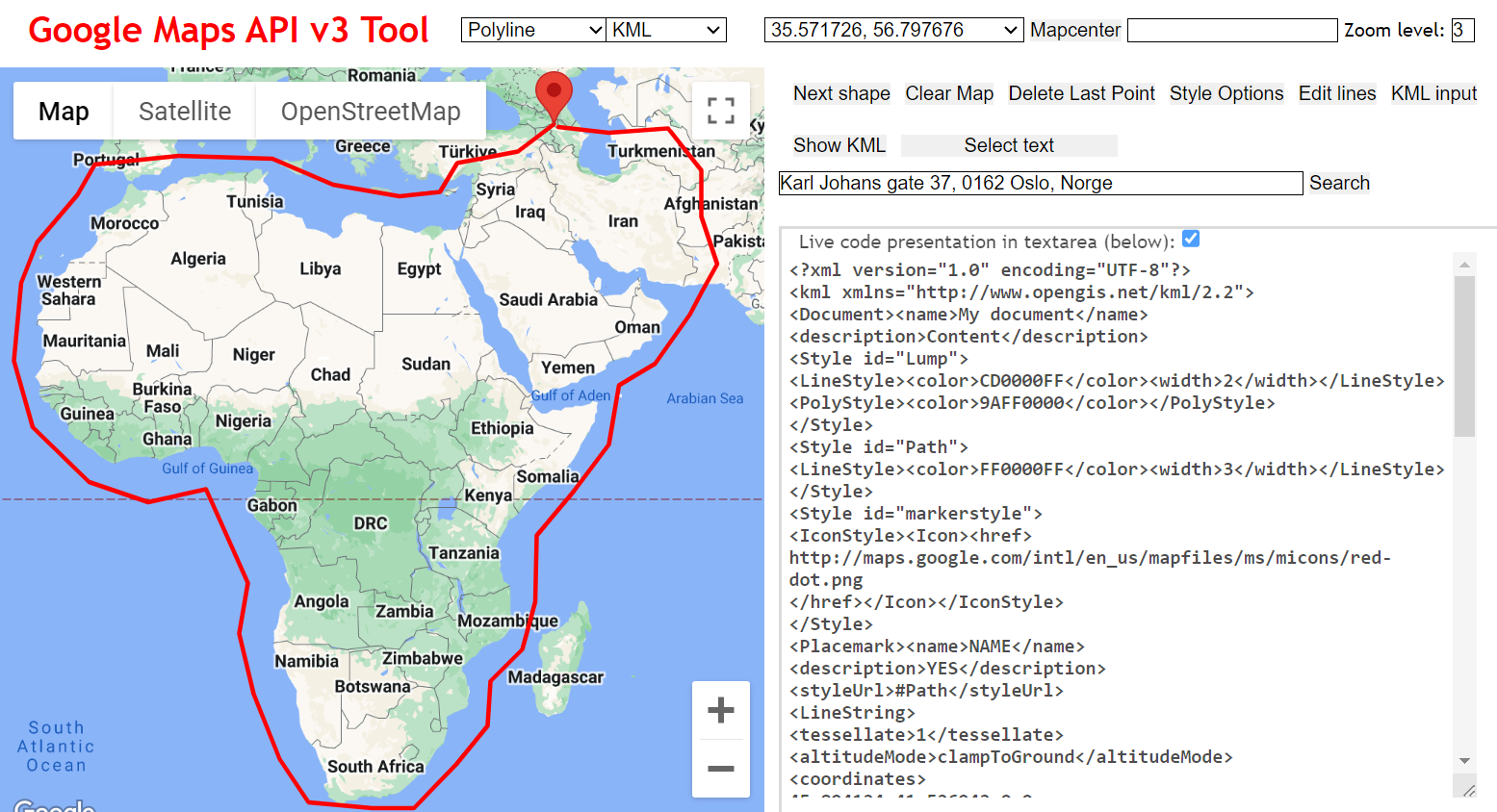
To save time, we’ve also prepare this file for you, and for this workshop you can simply download it.

!wget https://raw.githubusercontent.com/radcamp/radcamp.github.io/master/Kigali2023/Cheetah.coords
!wget https://raw.githubusercontent.com/radcamp/radcamp.github.io/master/Kigali2023/Cheetah.outer

Load the coordinates of the samples, the outline and the global shp file

# GPS Coordinates per sample in the same order as the genotypes
coord = np.loadtxt("./Cheetah.coords")
outer = np.loadtxt("./Cheetah.outer")
grid_path = "/home/osboxes/src/feems/feems/data/grid_250.shp"

# graph input files
outer, edges, grid, _ = prepare_graph_inputs(coord=coord, ggrid=grid_path, translated=False, buffer=0, outer=outer)

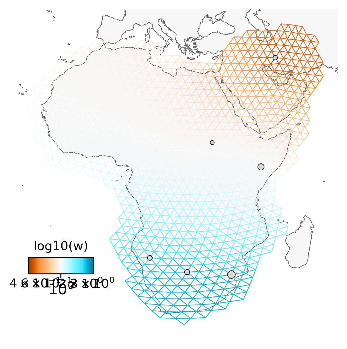
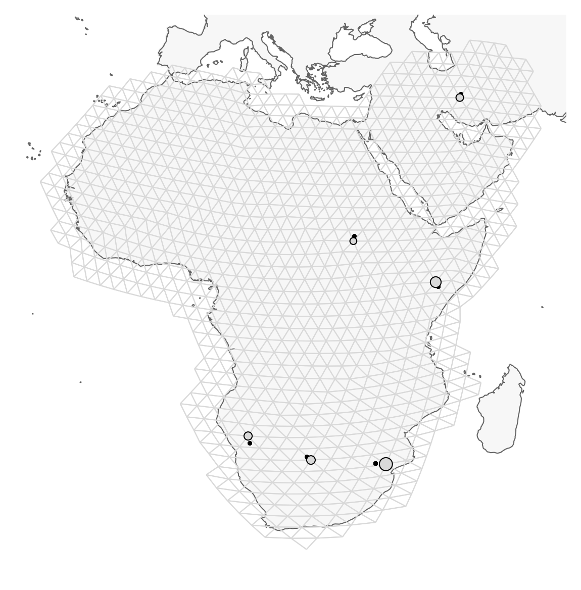
Plot the region and the sample sites

Note that the actual sampling locality is a small black dot, but for the analysis, it is locked to the grid and displayed as a grey circle (size depending on the number of samples). It is important to remember this, because it may look like sampling localities have changed. However, this is just because FEEMS makes it fit to the grid. This step may take a minute or so.

%%time
sp_graph = SpatialGraph(genotypes, coord, grid, edges, scale_snps=False)
projection = ccrs.EquidistantConic(central_longitude=23, central_latitude=8) 
fig = plt.figure(dpi=300) 
ax = fig.add_subplot(1, 1, 1, projection=projection) 
v = Viz(ax, sp_graph, projection=projection, edge_width=.5, 
    edge_alpha=1, edge_zorder=100, sample_pt_size=10, 
    obs_node_size=7.5, sample_pt_color="black", 
    cbar_font_size=10) 
v.draw_map() 
v.draw_samples() 
v.draw_edges(use_weights=False) 
v.draw_obs_nodes(use_ids=False) 

png

Fit the FEEMS model to the data

This step actually assesses to what degree genetic differentiation is higher or lower compared to what we can expect under IBD.

%%time 
sp_graph.fit(lamb = 20.0) 

Plot the fitted model

fig = plt.figure(dpi=300) 

ax = fig.add_subplot(1, 1, 1, projection=projection) 
v = Viz(ax, sp_graph, projection=projection, edge_width=0.5, 
    edge_alpha=1, edge_zorder=100, sample_pt_size=20, 
    obs_node_size=7.5, sample_pt_color="black", 
    cbar_font_size=10, abs_max=0.5) 
v.draw_map() 
v.draw_edges(use_weights=True) 
v.draw_obs_nodes(use_ids=False) 
v.draw_edge_colorbar() 

png