ipyrad command line assembly tutorial
This is the full tutorial for the command line interface (CLI) for ipyrad. In this tutorial we’ll walk through the entire assembly, from raw data to output files for downstream analysis. This is meant as a broad introduction to familiarize users with the general workflow, and some of the parameters and terminology. We will use and empirical dataset of paired-end cheetah ddRAD data as an example in this tutorial. Of course, you can replicate the steps described here with your own data, or any other RADseq dataset.
If you are new to RADseq analyses, this tutorial will provide a simple overview of how to execute ipyrad, what the data files look like, how to check that your analysis is working, and what the final output formats will be. We will also cover how to run ipyrad on a cluster and how to do so efficiently.
Each grey cell in this tutorial indicates a command line interaction.
Lines starting with $ indicate a command that should be executed in your terminal. All lines in code cells beginning with ## are
comments and should not be copied and executed. All other lines should
be interpreted as output from the issued commands.
Overview of Assembly Steps
Very roughly speaking, ipyrad exists to transform raw data coming off the sequencing instrument into output files that you can use for downstream analysis.
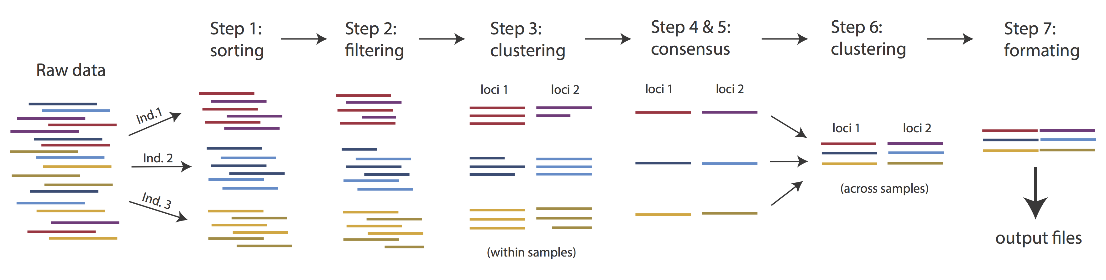
The basic steps of this process are as follows:
- Step 1 - Demultiplex/Load Raw Data
- Step 2 - Trim and Quality Control
- Step 3 - Cluster or reference-map within Samples
- Step 4 - Calculate Error Rate and Heterozygosity
- Step 5 - Call consensus sequences/alleles
- Step 6 - Cluster across Samples
- Step 7 - Apply filters and write output formats
Detailed information about ipyrad, including instructions for installation and troubleshooting, can be found here.
Note on files in the project directory: Assembling RADseq type sequence data requires a lot of different steps, and these steps generate a lot of intermediary files. ipyrad organizes these files into directories, and it prepends the name of your assembly to each directory with data that belongs to it. One result of this is that you can have multiple assemblies of the same raw data with different parameter settings and you don’t have to manage all the files yourself! (See Branching assemblies for more info). Another result is that you should not rename or move any of the directories inside your project directory, unless you know what you’re doing or you don’t mind if your assembly breaks.
Getting Started
We will be running through the assembly of the cheetah data using the ipyrad
CLI. So, if you don’t have the terminal window open, please start your VM, open a browser
window and navigate to http://localhost:8800 and create a new “Terminal”
using the “New” button.
ipyrad help
To better understand how to use ipyrad, let’s take a look at the help argument. We will use some of the ipyrad arguments in this tutorial (for example: -n, -p, -s, -c, -r). But, the complete list of optional arguments and their explanation is below.
(ipyrad) osboxes@osboxes:~/ipyrad-workshop$ ipyrad -h

usage: ipyrad [-h] [-v] [-r] [-f] [-q] [-d] [-n NEW] [-p PARAMS] [-s STEPS] [-b [BRANCH [BRANCH ...]]]
              [-m [MERGE [MERGE ...]]] [-c cores] [-t threading] [--MPI] [--ipcluster [IPCLUSTER]]
              [--download [DOWNLOAD [DOWNLOAD ...]]]

optional arguments:
  -h, --help            show this help message and exit
  -v, --version         show program's version number and exit
  -r, --results         show results summary for Assembly in params.txt and exit
  -f, --force           force overwrite of existing data
  -q, --quiet           do not print to stderror or stdout.
  -d, --debug           print lots more info to ipyrad_log.txt.
  -n NEW                create new file 'params-{new}.txt' in current directory
  -p PARAMS             path to params file for Assembly: params-{assembly_name}.txt
  -s STEPS              Set of assembly steps to run, e.g., -s 123
  -b [BRANCH [BRANCH ...]]
                        create new branch of Assembly as params-{branch}.txt, and can be used to drop samples from
                        Assembly.
  -m [MERGE [MERGE ...]]
                        merge multiple Assemblies into one joint Assembly, and can be used to merge Samples into one
                        Sample.
  -c cores              number of CPU cores to use (Default=0=All)
  -t threading          tune threading of multi-threaded binaries (Default=2)
  --MPI                 connect to parallel CPUs across multiple nodes
  --ipcluster [IPCLUSTER]
                        connect to running ipcluster, enter profile name or profile='default'
  --download [DOWNLOAD [DOWNLOAD ...]]
                        download fastq files by accession (e.g., SRP or SRR)

  * Example command-line usage:
    ipyrad -n data                       ## create new file called params-data.txt
    ipyrad -p params-data.txt -s 123     ## run only steps 1-3 of assembly.
    ipyrad -p params-data.txt -s 3 -f    ## run step 3, overwrite existing data.

  * HPC parallelization across 32 cores
    ipyrad -p params-data.txt -s 3 -c 32 --MPI

  * Print results summary
    ipyrad -p params-data.txt -r

  * Branch/Merging Assemblies
    ipyrad -p params-data.txt -b newdata
    ipyrad -m newdata params-1.txt params-2.txt [params-3.txt, ...]

  * Subsample taxa during branching
    ipyrad -p params-data.txt -b newdata taxaKeepList.txt

  * Download sequence data from SRA into directory 'sra-fastqs/'
    ipyrad --download SRP021469 sra-fastqs/

  * Documentation: http://ipyrad.readthedocs.io
Create a new parameters file
ipyrad uses a text file to hold all the parameters for a given assembly.
Start by creating a new parameters file with the -n flag. This flag
requires you to pass in a name for your assembly. In the example we use
cheetah but the name can be anything at all. Once you start
analysing your own data you might call your parameters file something
more informative, including some details on the
settings.
# Now create a new params file named 'cheetah'
(ipyrad) osboxes@osboxes:~/ipyrad-workshop$ ipyrad -n cheetah
This will create a file in the current directory called params-cheetah.txt.
The params file lists on each line one parameter followed by a ## mark,
then the name of the parameter, and then a short description of its purpose.
Lets take a look at it.
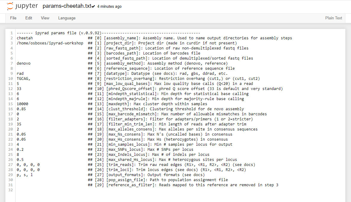
(ipyrad) osboxes@osboxes:~/ipyrad-workshop$ cat params-cheetah.txt
------- ipyrad params file (v.0.9.92)-------------------------------------------
cheetah                          ## [0] [assembly_name]: Assembly name. Used to name output directories for assembly steps
/home/osboxes//ipyrad-workshop   ## [1] [project_dir]: Project dir (made in curdir if not present)
                                 ## [2] [raw_fastq_path]: Location of raw non-demultiplexed fastq files
                                 ## [3] [barcodes_path]: Location of barcodes file
                                 ## [4] [sorted_fastq_path]: Location of demultiplexed/sorted fastq files
denovo                           ## [5] [assembly_method]: Assembly method (denovo, reference)
                                 ## [6] [reference_sequence]: Location of reference sequence file
rad                              ## [7] [datatype]: Datatype (see docs): rad, gbs, ddrad, etc.
TGCAG,                           ## [8] [restriction_overhang]: Restriction overhang (cut1,) or (cut1, cut2)
5                                ## [9] [max_low_qual_bases]: Max low quality base calls (Q<20) in a read
33                               ## [10] [phred_Qscore_offset]: phred Q score offset (33 is default and very standard)
6                                ## [11] [mindepth_statistical]: Min depth for statistical base calling
6                                ## [12] [mindepth_majrule]: Min depth for majority-rule base calling
10000                            ## [13] [maxdepth]: Max cluster depth within samples
0.85                             ## [14] [clust_threshold]: Clustering threshold for de novo assembly
0                                ## [15] [max_barcode_mismatch]: Max number of allowable mismatches in barcodes
0                                ## [16] [filter_adapters]: Filter for adapters/primers (1 or 2=stricter)
35                               ## [17] [filter_min_trim_len]: Min length of reads after adapter trim
2                                ## [18] [max_alleles_consens]: Max alleles per site in consensus sequences
0.05                             ## [19] [max_Ns_consens]: Max N's (uncalled bases) in consensus (R1, R2)
0.05                             ## [20] [max_Hs_consens]: Max Hs (heterozygotes) in consensus (R1, R2)
4                                ## [21] [min_samples_locus]: Min # samples per locus for output
0.2                              ## [22] [max_SNPs_locus]: Max # SNPs per locus (R1, R2)
8                                ## [23] [max_Indels_locus]: Max # of indels per locus (R1, R2)
0.5                              ## [24] [max_shared_Hs_locus]: Max # heterozygous sites per locus
0, 0, 0, 0                       ## [25] [trim_reads]: Trim raw read edges (R1>, <R1, R2>, <R2) (see docs)
0, 0, 0, 0                       ## [26] [trim_loci]: Trim locus edges (see docs) (R1>, <R1, R2>, <R2)
p, s, l                          ## [27] [output_formats]: Output formats (see docs)
                                 ## [28] [pop_assign_file]: Path to population assignment file
                                 ## [29] [reference_as_filter]: Reads mapped to this reference are removed in step 3
In general the defaults are sensible, and we won’t mess with them for now, but there are a few parameters we must check and update:
- The path to the raw data
- The dataype
- The restriction overhang sequence(s)
Because we’re looking at population-level data, we suggest to increase the clustering threshold [14] [clust_threshold]. You can also change [27] [output_formats]. When you put *, ipyrad will automatically save your output in all available formats, see the manual.
If you return to the browser tab with your jupyter notebook interface you’ll
now see a new file params-cheetah.txt in the file browser.
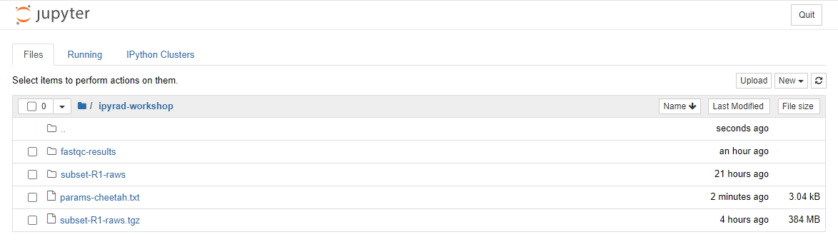
Clicking on this new file will open a text editor so you can modify and save changes to this params file.
We need to specify where the raw data files are located, the type of data we are using (.e.g., ‘gbs’, ‘rad’, ‘ddrad’, ‘pairddrad), and which enzyme cut site overhangs are expected to be present on the reads. Change the following lines in your params files to look like this:
./subset-R1-raws/*.fastq.gz     ## [4] [sorted_fastq_path]: Location of demultiplexed/sorted fastq files
CATGC                           ## [8] [restriction_overhang]: Restriction overhang (cut1,) or (cut1, cut2)
0.9                             ## [14] [clust_threshold]: Clustering threshold for de novo assembly
*                               ## [27] [output_formats]: Output formats (see docs)
NB: Don’t forget to choose “File->Save Text” after you are done editing!
Once we start running the analysis ipyrad will create several new directories to
hold the output of each step for this assembly. By default the new directories
are created in the project_dir directory and use the prefix specified by the
assembly_name parameter. For this example assembly all the intermediate
directories will be of the form: /ipyrad-workshop/cheetah_*.
Step 1: Loading/Demultiplexing the raw data
Sometimes, you’ll receive your data as a huge pile of reads, and you’ll need to
split it up and assign each read to the sample it came from. This is called
demultiplexing and is done by unique barcodes which allow you to recognize
individual samples. In that case, you’ll have to provide a path to the raw
non-demultiplexed fastq files [2] and the path to the barcode file [3] in
your params file. In our case, the samples are already demultiplexed and we have
1 file per sample. The path to these files is indicated in [4] in the params
file. Even though we do not need to demultiplex our data here, we still need to
run this step to import the data into ipyrad.
Note on step 1: If we would have data which need demultiplexing, Step 1 will create a new folder, called
cheetah_fastqs. Because our data are already demultiplexed, this folder will not be created.
Now lets run step 1!
Special Note: In some cases it’s useful to specify the number of cores with the
-cflag. If you do not specify the number of cores ipyrad assumes you want all of them.
## -p    the params file we wish to use
## -s    the step to run
## -c    run on 4 cores
(ipyrad) osboxes@osboxes:~/ipyrad-workshop$ ipyrad -p params-cheetah.txt -s 1 -c 4

 -------------------------------------------------------------
  ipyrad [v.0.9.92]
  Interactive assembly and analysis of RAD-seq data
 -------------------------------------------------------------
  Parallel connection | osboxes: 4 cores

  Step 1: Loading sorted fastq data to Samples
  [####################] 100% 0:00:13 | loading reads
  24 fastq files loaded to 24 Samples.
  Parallel connection closed.
In-depth operations of running an ipyrad step
Any time ipyrad is invoked it performs a few housekeeping operations:
- Load the assembly object - Since this is our first time running any steps we need to initialize our assembly.
- Start the parallel cluster - ipyrad uses a parallelization library called ipyparallel. Every time we start a step we fire up the parallel clients. This makes your assemblies go smokin’ fast.
- Do the work - Actually perform the work of the requested step(s) (in this case demultiplexing reads to samples).
- Save, clean up, and exit - Save the state of the assembly, and spin down the ipyparallel cluster.
As a convenience ipyrad internally tracks the state of all your steps in your
current assembly, so at any time you can ask for results by invoking the -r
flag. We also use the -p argument to tell it which params file (i.e., which
assembly) we want it to print stats for.
## -r fetches informative results from currently executed steps
(ipyrad) osboxes@osboxes:~/ipyrad-workshop$ ipyrad -p params-cheetah.txt -r
  loading Assembly: cheetah
  from saved path: ~/ipyrad-workshop/cheetah.json

Summary stats of Assembly cheetah
------------------------------------------------
              state  reads_raw
SRR19760910      1     125000
SRR19760912      1     125000
SRR19760918      1     125000
SRR19760920      1     125000
SRR19760921      1     125000
SRR19760924      1     125000
SRR19760927      1     125000
SRR19760928      1     125000
SRR19760942      1     125000
SRR19760946      1     125000
SRR19760947      1     125000
SRR19760949      1     125000
SRR19760950      1     125000
SRR19760951      1     125000
SRR19760953      1     120739
SRR19760954      1     125000
SRR19760955      1     125000
SRR19760956      1     125000
SRR19760957      1     125000
SRR19760958      1     125000
SRR19760959      1     125000
SRR19760960      1     125000
SRR19760961      1     125000
SRR19760962      1     125000


Full stats files
------------------------------------------------
step 1: ./cheetah_s1_demultiplex_stats.txt
step 2: None
step 3: None
step 4: None
step 5: None
step 6: None
step 7: None
If you want to get even more info, ipyrad tracks all kinds of wacky stats and saves them to a file inside the directories it creates for each step. For instance, to see full stats for step 1 (the wackyness of the step 1 stats at this point isn’t very interesting, but we’ll see stats for later steps are more verbose):
Step 2: Filter reads
This step filters reads based on quality scores and maximum number of uncalled bases, and can be used to detect Illumina adapters in your reads, which is sometimes a problem under a couple different library prep scenarios. We know the our data have an excess of low-quality bases toward the 5’ end (remember the FastQC results!), so lets use this opportunity to trim off some of those low quality regions. To account for this we will trim reads to 100bp, removing the last 10bp of our 110bp reads.
Edit your params file again with and change the following two parameter settings:
0, 100, 0, 0 ## [25] [trim_reads]: Trim raw read edges (R1>, <R1, R2>, <R2) (see docs)
(ipyrad) osboxes@osboxes:~/ipyrad-workshop$ ipyrad -p params-cheetah.txt -s 2 -c 4
  loading Assembly: cheetah
  from saved path: ~/ipyrad-workshop/cheetah.json

 -------------------------------------------------------------
  ipyrad [v.0.9.92]
  Interactive assembly and analysis of RAD-seq data
 -------------------------------------------------------------
  Parallel connection | osboxes: 4 cores

  Step 2: Filtering and trimming reads
  [####################] 100% 0:01:29 | processing reads

  Parallel connection closed.
The filtered files are written to a new directory called cheetah_edits. Again,
you can look at the results from this step and some handy stats tracked
for this assembly.
## View the output of step 2
(ipyrad) osboxes@osboxes:~/ipyrad-workshop$ cat cheetah_edits/s2_rawedit_stats.txt
      reads_raw  trim_adapter_bp_read1  trim_adapter_bp_read2  trim_quality_bp_read1  trim_quality_bp_read2  reads_filtered_by_Ns  reads_filtered_by_minlen  reads_passed_filter
reads_raw  trim_adapter_bp_read1  trim_quality_bp_read1  reads_filtered_by_Ns  reads_filtered_by_minlen  reads_passed_filter
SRR19760910     125000                   3907                 151184                    59                       266               124675
SRR19760912     125000                   4316                 232833                    65                       631               124304
SRR19760918     125000                   4029                  44448                     3                        37               124960
SRR19760920     125000                   3981                  46216                     5                        47               124948
SRR19760921     125000                   4140                  45663                    14                        31               124955
SRR19760924     125000                   4355                  42285                     9                        47               124944
SRR19760927     125000                   4120                  51549                    11                        52               124937
SRR19760928     125000                   4068                  44598                     8                        46               124946
SRR19760942     125000                   4210                  48041                    12                       250               124738
SRR19760946     125000                   4538                  39388                     9                       390               124601
SRR19760947     125000                   4335                  44185                    14                        39               124947
SRR19760949     125000                   4383                 187211                    55                       313               124632
SRR19760950     125000                   3757                 184015                    52                       393               124555
SRR19760951     125000                   3956                 261547                    62                       677               124261
SRR19760953     120739                   4097                 119160                    49                       268               120422
SRR19760954     125000                   4176                 238676                    56                       639               124305
SRR19760955     125000                   3783                 241923                    56                       584               124360
SRR19760956     125000                   4290                 178120                    63                       379               124558
SRR19760957     125000                   4068                 191626                    49                       410               124541
SRR19760958     125000                   4290                 177849                    65                       354               124581
SRR19760959     125000                   4027                 221129                    74                       523               124403
SRR19760960     125000                   4127                 171203                    60                       316               124624
SRR19760961     125000                   3976                 254342                    46                       640               124314
SRR19760962     125000                   3948                 220764                    52                       530               124418
## Get current stats including # raw reads and # reads after filtering.
(ipyrad) osboxes@osboxes:~/ipyrad-workshop$ ipyrad -p params-cheetah.txt -r
You might also take a closer look at the filtered reads:
(ipyrad) osboxes@osboxes:~/ipyrad-workshop$ zcat cheetah_edits/SRR19760910.trimmed_R1_.fastq.gz | head -n 12
@SRR19760910.1 1 length=110
CATGCACGTGCAGCATATAAGAAGGATGTTTGTCATGCATTATCTTATTTGATGTTTACGGAAGCCCCATGGTTATCCCCATTTTAGGGATGAAGAAACG
+
BFFFFFF<FBFFFFFF<FB//////<<FFFBFF//<FFFFFFBF/FBFFFFFFFFFFFFBB<F/BFFFFFFFFBFF/<<</BFBBFF/<FF<FF<7FFFF
@SRR19760910.2 2 length=110
CATGCAACTCTTGGTCTCGGGGTCTTGAGTTCGAGCCCCACGTTGGATTAGAGATTACTTAAATAAATAAAGTTCAAAAGTTTTAGAATGTTATCATTTT
+
FFFFFFFFFFFFFFFFFFFFFFFFFFFFFFFFFFFFFFFFFFFFFFFFFFFFFFFFFFFFFFFFFFFFFFFFFFFFFFFFFFFFFFFFFFFFFFFFFFFF
@SRR19760910.3 3 length=110
CATGCCATTTCCCATGGGCAAGGATCTCAGGCTGTGCTCATTCCCAAGGACAAGACCAAGCCAATTCCCAATCCCCATATTTAAGGAGCTGCTTCCTGGG
+
FFFFFFFFFFFFFFFFFFFFFFFFFFFFFFFFF<FFFFFFFFFFFFFFFBFFFFFFFFFFFFFFFFFFFFFFFFFFBFFFFFFFFFBFFFFFFFFFFFFF
This is actually really cool, because we can already see the results of our applied parameters. All reads have been trimmed to 100bp.
Step 3: denovo clustering within-samples
For a de novo assembly, step 3 de-replicates and then clusters reads within
each sample by the set clustering threshold and then writes the clusters to new
files in a directory called cheetah_clust_0.9. Intuitively, we are trying to
identify all the reads that map to the same locus within each sample. You may
remember the default value is 0.85, but we have increased if to 0.9 in our
params file. This value dictates the percentage of sequence similarity that
reads must have in order to be considered reads at the same locus.
NB: The true name of this output directory will be dictated by the value you set for the
clust_thresholdparameter in the params file.
You’ll more than likely want to experiment with this value, but 0.9 is a reasonable default for population genetic-scale data, balancing over-splitting of loci vs over-lumping. Don’t mess with this until you feel comfortable with the overall workflow, and also until you’ve learned about branching assemblies.
NB: What is the best clustering threshold to choose? “It depends.”
It’s also possible to incorporate information from a reference genome to improve clustering at this step, if such a resources is available for your organism (or one that is relatively closely related). We will not cover reference based assemblies in this workshop, but you can refer to the ipyrad documentation for more information.
Note on performance: Steps 3 and 6 generally take considerably longer than any of the steps, due to the resource intensive clustering and alignment phases. These can take on the order of 10-100x as long as the next longest running step. This depends heavily on the number of samples in your dataset, the number of cores, the length(s) of your reads, and the “messiness” of your data.
Now lets run step 3:
(ipyrad) osboxes@osboxes:~/ipyrad-workshop$ ipyrad -p params-cheetah.txt -s 3 -c 4
  loading Assembly: cheetah
  from saved path: ~/ipyrad-workshop/cheetah.json

 -------------------------------------------------------------
  ipyrad [v.0.9.92]
  Interactive assembly and analysis of RAD-seq data
 -------------------------------------------------------------
  Parallel connection | osboxes: 4 cores

  Step 3: Clustering/Mapping reads within samples
  [####################] 100% 0:00:13 | dereplicating
  [####################] 100% 0:09:46 | clustering/mapping
  [####################] 100% 0:00:00 | building clusters
  [####################] 100% 0:00:00 | chunking clusters
  [####################] 100% 0:16:25 | aligning clusters
  [####################] 100% 0:00:59 | concat clusters
  [####################] 100% 0:00:05 | calc cluster stats

  Parallel connection closed.
In-depth operations of step 3:
- dereplicating - Merge all identical reads
- clustering - Find reads matching by sequence similarity threshold
- building clusters - Group similar reads into clusters
- chunking clusters - Subsample cluster files to improve performance of alignment step
- aligning clusters - Align all clusters
- concat clusters - Gather chunked clusters into one full file of aligned clusters
- calc cluster stats - Just as it says.
Again we can examine the results. The stats output tells you how many clusters were found (‘clusters_total’), and the number of clusters that pass the mindepth thresholds (‘clusters_hidepth’). We’ll go into more detail about mindepth settings in some of the advanced tutorials.
(ipyrad) osboxes@osboxes:~/ipyrad-workshop$ ipyrad -p params-cheetah.txt -r
Summary stats of Assembly cheetah
------------------------------------------------
             state  reads_raw  reads_passed_filter  clusters_total  clusters_hidepth
SRR19760910      3     125000               124675           36092              6433
SRR19760912      3     125000               124304           38568              6103
SRR19760918      3     125000               124960           34586              6989
SRR19760920      3     125000               124948           34759              6851
SRR19760921      3     125000               124955           34423              7003
SRR19760924      3     125000               124944           35112              6793
SRR19760927      3     125000               124937           34872              6941
SRR19760928      3     125000               124946           35102              6860
SRR19760942      3     125000               124738           36514              6629
SRR19760946      3     125000               124601           40697              6135
SRR19760947      3     125000               124947           37190              6262
SRR19760949      3     125000               124632           37495              6179
SRR19760950      3     125000               124555           33231              6092
SRR19760951      3     125000               124261           33844              6744
SRR19760953      3     120739               120422           33549              6216
SRR19760954      3     125000               124305           35873              6326
SRR19760955      3     125000               124360           33113              6186
SRR19760956      3     125000               124558           39780              5953
SRR19760957      3     125000               124541           37946              6190
SRR19760958      3     125000               124581           38539              6043
SRR19760959      3     125000               124403           38225              6172
SRR19760960      3     125000               124624           38138              6238
SRR19760961      3     125000               124314           36710              6333
SRR19760962      3     125000               124418           33510              7085

Full stats files
------------------------------------------------
step 1: ./cheetah_s1_demultiplex_stats.txt
step 2: ./cheetah_edits/s2_rawedit_stats.txt
step 3: ./cheetah_clust_0.9/s3_cluster_stats.txt
step 4: None
step 5: None
step 6: None
step 7: None
Again, the final output of step 3 is dereplicated, clustered files for
each sample in ./cheetah_clust_0.9/. You can get a feel for what
this looks like by examining a portion of one of the files.
## Same as above, `zcat` unzips and prints to the screen and
## `head -n 18` means just show me the first 18 lines.
(ipyrad) osboxes@osboxes:~/ipyrad-workshop$t zcat cheetah_clust_0.9/SRR19760910.clustS.gz | head -n 18
You’ll see something similar to what is printed below:
0121ac19c8acb83e5d426007a2424b65;size=18;*
TGCAGTTGGGATGGCGATGCCGTACATTGGCGCATCCAGCCTCGGTCATTGTCGGAGATCTCACCTTTCAACGGTnnnnTGAATGGTCGCGACCCCCAACCACAATCGGCTTTGCCAAGGCAAGGCTAGAGACGTGCTAAAAAAACTCGCTCCG
521031ed2eeb3fb8f93fd3e8fdf05a5f;size=1;+
TGCAGTTGGGATGGCGATGCCGTACATTGGCGCATCCAGCCTCGGTCATTGTCGGAGATCTCACCTTTCAACGGTnnnnTGAATGGTCGCGACCCCCAACCACAATCGGCTTTGCCAAGGCAAGGCTAGAGAAGTGCTAAAAAAACTCGCTCCG
//
//
014947fbb43ef09f5388bbd6451bdca0;size=12;*
TGCAGGACTGCGAATGACGGTGGCTAGTACTCGAGGAAGGGTCGCACCGCAGTAAGCTAATCTGACCCTCTGGAGnnnnACCAGTGGTGGGTAAACACCTCCGATTAAGTATAACGCTACGTGAAGCTAAACGGCACCTATCACATAGACCCCG
072588460dac78e9da44b08f53680da7;size=8;+
TGCAGGTCTGCGAATGACGGTGGCTAGTACTCGAGGAAGGGTCGCACCGCAGTAAGCTAATCTGACCCTCTGGAGnnnnACCAGTGGTGGGTAAACACCTCCGATTAAGTATAACGCTACGTGAAGCTAAACGGCACCTATCACATAGACCCCG
fce2e729af9ea5468bafbef742761a4b;size=1;+
TGCAGGACTGCGAATGACGGTGGCTAGTACTCGAGGAAGGGTCGCACCGCAGCAAGCTAATCTGACCCTCTGGAGnnnnACCAGTGGTGGGTAAACACCTCCGATTAAGTATAACGCTACGTGAAGCTAAACGGCACCTATCACATAGACCCCG
24d23e93688f17ab0252fe21f21ce3a7;size=1;+
TGCAGGTCTGCGAATGACGGTGGCTAGTACTCGAGGAAGGGTCGCACCGCAGAAAGCTAATCTGACCCTCTGGAGnnnnACCAGTGGTGGGTAAACACCTCCGATTAAGTATAACGCTACGTGAAGCTAAACGGCACCTATCACATAGACCCCG
ef2c0a897eb5976c40f042a9c3f3a8ba;size=1;+
TGCAGGTCTGCGAATGACGGTGGCTAGTACTCGAGGAAGGGTCGCACCGCAGTAAGCTAATCTGACCCTCTGGAGnnnnACCAGTGGTGGGTAAACACCTCCGATTAAGTATAACGCTACGTGAAGCTAAACGGCACCTATCACATCGACCCCG
//
//
Reads that are sufficiently similar (based on the above sequence similarity threshold) are grouped together in clusters separated by “//”. The first cluster above is probably homozygous with some sequencing error. The second cluster is probably heterozygous with some sequencing error. We don’t want to go through and ‘decide’ by ourselves for each cluster, so thankfully, untangling this mess is what steps 4 & 5 are all about.
Step 4: Joint estimation of heterozygosity and error rate
In Step 3 reads that are sufficiently similar (based on the specified sequence
similarity threshold) are grouped together in clusters separated by “//”. We
examined the head of one of the sample cluster files at the end of the last
exercise, but here we’ve cherry picked a couple clusters with more pronounced
features.
Here’s a nice homozygous cluster, with probably one read with sequencing error:
0082e23d9badff5470eeb45ac0fdd2bd;size=5;*
TGCATGTAGTGAAGTCCGCTGTGTACTTGCGAGAGAATGAGTAGTCCTTCATGCA
a2c441646bb25089cd933119f13fb687;size=1;+
TGCATGTAGTGAAGTCCGCTGTGTACTTGCGAGAGAATGAGCAGTCCTTCATGCA
Here’s a probable heterozygote, or perhaps repetitive element – a little bit messier (note the indels):
0091f3b72bfc97c4705b4485c2208bdb;size=3;*
TGCATACAC----GCACACA----GTAGTAGTACTACTTTTTGTTAACTGCAGCATGCA
9c57902b4d8e22d0cda3b93f1b361e78;size=3;-
TGCATACAC----ACACACAACCAGTAGTAGTATTACTTTTTGTTAACTGCAGCATGCA
d48b3c7b5a0f1840f54f6c7808ca726e;size=1;+
TGCATACAC----ACAAACAACCAGTTGTAGTACTACTTTTTGTTAACTGCAGCATGAA
fac0c64aeb8afaa5dfecd5254b81b3c0;size=1;+
TGCATACAC----GCACACAACCAGTAGTAGTACTACTTTTTGTTAACTGCAGCATGTA
f31cbca6df64e7b9cb4142f57e607a88;size=1;-
TGCATGCACACACGCACGCAACCAGTAGTTGTACTACTTTTTGTTAACTGCAGCATGCA
935063406d92c8c995d313b3b22c6484;size=1;-
TGCATGCATACACGCCCACAACCAGTAGTAGTACAACTTTATGTTAACTGCAGCATGCA
d25fcc78f14544bcb42629ed2403ce74;size=1;+
TGCATACAC----GCACACAACCAGTAGTAGTACTACTTTTTGTTAATTGCAGCATGCA
Here’s a nasty one!
008a116c7a22d6af3541f87b36a8d895;size=3;*
TGCATTCCTATGGGAATCATGAAGGGGCTTCTCTCTCCCTCA-TTTTTAAAGCGACCCTTTCCAAACTTGGTACAT----
a7bde31f2034d2e544400c62b1d3cbd5;size=2;+
TGCATTCCTATGGGAAACATGAAGGGACTTCTCTCTCCCTCG-TTTTTAAAGTGACTCTGTCCAAACTTGGTACAT----
107e1390e1ac8564619a278fdae3f009;size=2;+
TGCATTCCTATGGGAAACATGAAGGGGGTTCTCTCTCCCTCG-ATTTTAAAGCGACCCTGTCCAAACTTGGTACAT----
8f870175fb30eed3027b7aec436e93e6;size=2;+
TGCATTCCTATGGGAATCATGGAAGGGCTTCTCTCTCCCTCA-TTTTTAAAGCAACCCTGACCAAAGTTGGTACAT----
445157bc1e7540734bf963eb8629d827;size=2;+
TGCATTCCTACGGGAATCATGGAGGGGCTTCTCTCTCCCTCG-TTTTTAAAGCGACCCTGACCAAACTTGGTACAT----
9ddd2d8b6fb52157f17648682d09afda;size=1;+
TGCATTCCTATGAGAAACATGATGGGGCTTCTCTTTCCCTCATTTTTT--AGTTAGCCTTACCAAAGTTGGTACATT---
fc86d48758313be18587d6f185e5c943;size=1;+
TGCATTCCTGTGGGAAACATGAAGGGGCTTCTCTCTCCATCA-TTTTTAAAGCGACCCTGATCAAATTTGGTACAT----
243a5acbee6cd9cd223252a8bb65667e;size=1;+
TGCATTCCTATGGGAAACATGAAAGGGTTTCTCTCTCCCTCG-TTTTAAAAGCGACCCTGTCCAAACATGGTACAT----
55e50e131ec21fce8021f22de49bb7be;size=1;+
TGCATTCCAATGGGAAACATGAAAGGGCTTCTCTCTCCCTCG-TTTTTAAAGCGACCCTGTCCAAACTTGGTACAT----
For this final cluster it’s really hard to call by eye, that’s why we make the computer do it!
In this step we jointly estimate sequencing error rate and heterozygosity to help us figure out which reads are “real” and which include sequencing error. We need to know which reads are “real” because in diploid organisms there are a maximum of 2 alleles at any given locus. If we look at the raw data and there are 20 different “alleles”, and 2 of them are very high frequency, and the rest are singletons then this gives us evidence that the 2 high frequency alleles are the good reads and the rest are probably junk. This step is pretty straightforward, and pretty fast. Run it like this:
(ipyrad) osboxes@osboxes:~/ipyrad-workshop$ ipyrad -p params-cheetah.txt -s 4 -c 4
  loading Assembly: cheetah
  from saved path: ~/ipyrad-workshop/cheetah.json

 -------------------------------------------------------------
  ipyrad [v.0.9.92]
  Interactive assembly and analysis of RAD-seq data
 -------------------------------------------------------------
  Parallel connection | osboxes: 4 cores

  Step 4: Joint estimation of error rate and heterozygosity
  [####################] 100% 0:01:46 | inferring [H, E]

  Parallel connection closed.
In terms of results, there isn’t as much to look at as in previous steps, though
you can invoke the -r flag to see the estimated heterozygosity and error rate
per sample.
(ipyrad) osboxes@osboxes:~/ipyrad-workshop$ ipyrad -p params-cheetah.txt -r
Summary stats of Assembly cheetah
------------------------------------------------
             state  reads_raw  reads_passed_filter  clusters_total  clusters_hidepth  hetero_est  error_est
SRR19760910      4     125000               124675           36092              6433    0.001586   0.001939
SRR19760912      4     125000               124304           38568              6103    0.001574   0.001457
SRR19760918      4     125000               124960           34586              6989    0.001941   0.001793
SRR19760920      4     125000               124948           34759              6851    0.001958   0.001718
SRR19760921      4     125000               124955           34423              7003    0.001757   0.001781
SRR19760924      4     125000               124944           35112              6793    0.001780   0.001774
SRR19760927      4     125000               124937           34872              6941    0.001694   0.001987
SRR19760928      4     125000               124946           35102              6860    0.001663   0.001771
SRR19760942      4     125000               124738           36514              6629    0.001523   0.001638
SRR19760946      4     125000               124601           40697              6135    0.001910   0.001771
SRR19760947      4     125000               124947           37190              6262    0.002124   0.001934
SRR19760949      4     125000               124632           37495              6179    0.002958   0.001242
SRR19760950      4     125000               124555           33231              6092    0.000969   0.001323
SRR19760951      4     125000               124261           33844              6744    0.001339   0.001439
SRR19760953      4     120739               120422           33549              6216    0.001850   0.002019
SRR19760954      4     125000               124305           35873              6326    0.001581   0.001559
SRR19760955      4     125000               124360           33113              6186    0.001643   0.001609
SRR19760956      4     125000               124558           39780              5953    0.001578   0.001316
SRR19760957      4     125000               124541           37946              6190    0.001664   0.001254
SRR19760958      4     125000               124581           38539              6043    0.001611   0.001330
SRR19760959      4     125000               124403           38225              6172    0.001353   0.001430
SRR19760960      4     125000               124624           38138              6238    0.001306   0.001118
SRR19760961      4     125000               124314           36710              6333    0.001388   0.001479
SRR19760962      4     125000               124418           33510              7085    0.001505   0.001343


Full stats files
------------------------------------------------
step 1: ./cheetah_s1_demultiplex_stats.txt
step 2: ./cheetah_edits/s2_rawedit_stats.txt
step 3: ./cheetah_clust_0.9/s3_cluster_stats.txt
step 4: ./cheetah_clust_0.9/s4_joint_estimate.txt
step 5: None
step 6: None
step 7: None
Illumina error rates are on the order of 0.1% per base, so your error rates will ideally be in this neighborhood. Also, under normal conditions error rate will be much, much lower than heterozygosity (on the order of 10x lower). If the error rate is »0.1% then you might be using too permissive a clustering threshold. Just a thought.
Step 5: Consensus base calls
Step 5 uses the inferred error rate and heterozygosity per sample to call the consensus of sequences within each cluster. Here we are identifying what we believe to be the real haplotypes at each locus within each sample.
(ipyrad) osboxes@osboxes:~/ipyrad-workshop$ ipyrad -p params-cheetah.txt -s 5 -c 4
  loading Assembly: cheetah
  from saved path: ~/ipyrad-workshop/cheetah.json

 -------------------------------------------------------------
  ipyrad [v.0.9.92]
  Interactive assembly and analysis of RAD-seq data
 -------------------------------------------------------------
  Parallel connection | osboxes: 4 cores

  Step 5: Consensus base/allele calling
  Mean error  [0.00158 sd=0.00026]
  Mean hetero [0.00168 sd=0.00037]
  [####################] 100% 0:00:04 | calculating depths
  [####################] 100% 0:00:05 | chunking clusters
  [####################] 100% 0:10:05 | consens calling
  [####################] 100% 0:00:19 | indexing alleles

  Parallel connection closed.
In-depth operations of step 5:
- calculating depths - A simple refinement of the H/E estimates
- chunking clusters - Again, breaking big files into smaller chunks to aid parallelization
- consensus calling - Actually perform the consensus sequence calling
- indexing alleles - Cleaning up and re-joining chunked data
(ipyrad) osboxes@osboxes:~/ipyrad-workshop$ ipyrad -p params-cheetah.txt -r
  loading Assembly: cheetah
  from saved path: ~/ipyrad-workshop/cheetah.json

Summary stats of Assembly cheetah
------------------------------------------------
             state  reads_raw  reads_passed_filter  clusters_total  clusters_hidepth  hetero_est  error_est  reads_consens
SRR19760910      5     125000               124675           36092              6433    0.001586   0.001939           6355
SRR19760912      5     125000               124304           38568              6103    0.001574   0.001457           6036
SRR19760918      5     125000               124960           34586              6989    0.001941   0.001793           6905
SRR19760920      5     125000               124948           34759              6851    0.001958   0.001718           6766
SRR19760921      5     125000               124955           34423              7003    0.001757   0.001781           6930
SRR19760924      5     125000               124944           35112              6793    0.001780   0.001774           6724
SRR19760927      5     125000               124937           34872              6941    0.001694   0.001987           6867
SRR19760928      5     125000               124946           35102              6860    0.001663   0.001771           6793
SRR19760942      5     125000               124738           36514              6629    0.001523   0.001638           6566
SRR19760946      5     125000               124601           40697              6135    0.001910   0.001771           6072
SRR19760947      5     125000               124947           37190              6262    0.002124   0.001934           6182
SRR19760949      5     125000               124632           37495              6179    0.002958   0.001242           6090
SRR19760950      5     125000               124555           33231              6092    0.000969   0.001323           6043
SRR19760951      5     125000               124261           33844              6744    0.001339   0.001439           6677
SRR19760953      5     120739               120422           33549              6216    0.001850   0.002019           6142
SRR19760954      5     125000               124305           35873              6326    0.001581   0.001559           6255
SRR19760955      5     125000               124360           33113              6186    0.001643   0.001609           6102
SRR19760956      5     125000               124558           39780              5953    0.001578   0.001316           5897
SRR19760957      5     125000               124541           37946              6190    0.001664   0.001254           6124
SRR19760958      5     125000               124581           38539              6043    0.001611   0.001330           5976
SRR19760959      5     125000               124403           38225              6172    0.001353   0.001430           6117
SRR19760960      5     125000               124624           38138              6238    0.001306   0.001118           6178
SRR19760961      5     125000               124314           36710              6333    0.001388   0.001479           6269
SRR19760962      5     125000               124418           33510              7085    0.001505   0.001343           7018


Full stats files
------------------------------------------------
step 1: ./cheetah_s1_demultiplex_stats.txt
step 2: ./cheetah_edits/s2_rawedit_stats.txt
step 3: ./cheetah_clust_0.9/s3_cluster_stats.txt
step 4: ./cheetah_clust_0.9/s4_joint_estimate.txt
step 5: ./cheetah_consens/s5_consens_stats.txt
step 6: None
step 7: None
And here the important information is the number of reads_consens. This is
the number of retained reads within each sample that we’ll send on to the next
step. Retained reads must pass filters on read depth tolerance (both
mindepth_majrule and maxdepth), maximum number of uncalled bases
(max_Ns_consens) and maximum number of heterozygous sites (max_Hs_consens)
per consensus sequence. This number will almost always be lower than
clusters_hidepth.
Step 6: Cluster across samples
Step 6 clusters consensus sequences across samples. Now that we have good estimates for haplotypes within samples we can try to identify similar sequences at each locus among samples. We use the same clustering threshold as step 3 to identify sequences among samples that are probably sampled from the same locus, based on sequence similarity.
Note on performance of each step: Again, step 6 can take some time for large empirical datasets, but it’s normally faster than step 3.
(ipyrad) osboxes@osboxes:~/ipyrad-workshop$ ipyrad -p params-cheetah.txt -s 6 -c 4
  loading Assembly: cheetah
  from saved path: ~/ipyrad-workshop/cheetah.json

 -------------------------------------------------------------
  ipyrad [v.0.9.92]
  Interactive assembly and analysis of RAD-seq data
 -------------------------------------------------------------
  Parallel connection | osboxes: 4 cores

  Step 6: Clustering/Mapping across samples
  [####################] 100% 0:00:03 | concatenating inputs
  [####################] 100% 0:01:18 | clustering across
  [####################] 100% 0:00:06 | building clusters
  [####################] 100% 0:02:55 | aligning clusters

  Parallel connection closed.
In-depth operations of step 6:
- concatenating inputs - Gathering all consensus files and preprocessing to improve performance.
- clustering across - Cluster by similarity threshold across samples
- building clusters - Group similar reads into clusters
- aligning clusters - Align within each cluster
Since in general the stats for results of each step are sample based, the output
of -r will only display what we had seen after step 5, so this is not that
informative.
It might be more enlightening to consider the output of step 6 by examining the file that contains the reads clustered across samples:
(ipyrad) osboxes@osboxes:~/ipyrad-workshop$ cat cheetah_across/cheetah_clust_database.fa | head -n 27
>SRR19760910_0
CATGCATCTAAAATTATAGAGTACTCATGTTTTACAAAGGAATTCAGCCTGTTTTACAAACACATCAGGTGAGCATCACCCACCTTAGCTAATGTTATGG
>SRR19760912_0
CATGCATCTAAAATTATAGAGTACTCATGTTTTACAAAGGAATTCAGCCTGTTTTACAAACACATCAGGTGAGCATCACCCACCTTAGCTAATGTTATGG
>SRR19760919_1
CATGCATCTAAAATTATAGAGTACTCATGTTTTACAAAGGAATTCAGCCTGTTTTACAAACACATCAGGTGAGCATCACCCACCTTAGCTAATGTTATGG
>SRR19760947_0
CATGCATCTAAAATTATAGAGTACTCATGTTTTACAAAGGAATTCAGCCTGTTTTACAAACACATCAGGTGAGCATCACCCACCTTAGCTAATGTTATGG
>SRR19760951_1
CATGCATCTAAAATTATAGAGTACTCATGTTTTACAAAGGAATTCAGCCTGTTTTACAAACACATCAGGTGAGCATCACCCACCTTAGCTAATGTTATGG
>SRR19760954_5064
CATGCATCTAAAATTATAGAGTACTCATGTTTTACAAAGGAATTCAGCCTGTTTTACAAACACATCAGGTGAGCATCACCCACCTTAGCTAATGTTATGG
>SRR19760957_5406
CATGCATCTAAAATTATAGAGTACTCATGTTTTACAAAGGAATTCAGCCTGTTTTACAAACACATCAGGTGAGCATCACCCACCTTAGCTAATGTTATGG
>SRR19760961_5265
CATGCATCTAAAATTATAGAGTACTCATGTTTTACAAAGGAATTCAGCCTGTTTTACAAACACATCAGGTGAGCATCACCCACCTTAGCTAATGTTATGG
//
//
>SRR19760910_10
CATGCTCTGCTCTGCAGCCTGCAGTCTTTATGTTTGCTCTATGTCATAAGAATTCTGGCATACTTGTTTCTGTGAAATACCTGTATTTAGAGAACAGACG
>SRR19760911_4305
CATGCTCTGCTCTGCAGCCTGCAGTCTTTATGTTTGCTCTATGTCATAAGAATTCTGGCATACTTGTTTCTGTGAAATACCTGTATTTAGAGAACAGACG
>SRR19760913_9
CATGCTCTGCTCTGCAGCCTGCAGTCTTTATGTTTGCTCTATGTCATAAGAATTCTGGCATACTTGTTTCTGTGAAATACCTGTATTTAGAGAACAGACG
>SRR19760920_12
CATGCTCTGCTCTGCAGCCTGCAGTCTTTATGTTTGCTCTATGTCATAAGAATTCTGGCATACTTGTTTCTGTGAAATACCTGTATTTAGAGAACAGACG
>SRR19760921_14
CATGCTCTGCTCTGCAGCCTGCAGTCTTTATGTTTGCTCTATGTCATAAGAATTCTGGCATACTTGTTTCTGTGAAATACCTGTATTTAGAGAACAGACG
>SRR19760951_11
CATGCTCTGCTCTGCAGCCTGCAGTCTTTATGTTTGCTCTATGTCATAAGAATTCTGGCATACTTGTTTCTGTGAAATACCTGTATTTAGAGAACAGACG
>SRR19760952_11
CATGCTCTGCTCTGCAGCCTGCAGTCTTTATGTTTGCTCTATGTCATAAGAATTCTGGCATACTTGTTTCTGTGAAATACCTGTATTTAGAGAACAGACG
>SRR19760957_12
CATGCTCTGCTCTGCAGCCTGCAGTCTTTATGTTTGCTCTATGTCATAAGAATTCTGGCATACTTGTTTCTGTGAAATACCTGTATTTAGAGAACAGACG
>SRR19760958_8
CATGCTCTGCTCTGCAGCCTGCAGTCTTTATGTTTGCTCTATGTCATAAGAATTCTGGCATACTTGTTTCTGTGAAATACCTGTATTTAGAGAACAGACG
>SRR19760962_9
CATGCTCTGCTCTGCAGCCTGCAGTCTTTATGTTTGCTCTATGTCATAAGAATTCTGGCATACTTGTTTCTGTGAAATACCTGTATTTAGAGAACAGACG
//
//
The final output of step 6 is a file in cheetah_across called
cheetah_clust_database.fa. This file contains all aligned reads across all
samples. Executing the above command you’ll see all the reads that align at
each locus. You’ll see the sample name of each read followed by the sequence of
the read at that locus for that sample. If you wish to examine more loci you
can increase the number of lines you want to view by increasing the value you
pass to head in the above command (e.g. ... | head -n 300).
Step 7: Filter and write output files
The final step is to filter the data and write output files in many convenient file formats. First, we apply filters for maximum number of indels per locus, max heterozygosity per locus, max number of snps per locus, and minimum number of samples per locus. All these filters are configurable in the params file. You are encouraged to explore different settings, but the defaults are quite good and quite conservative.
To run step 7:
(ipyrad) osboxes@osboxes:~/ipyrad-workshop$ ipyrad -p params-cheetah.txt -s 7 -c 4
  loading Assembly: cheetah
  from saved path: ~/ipyrad-workshop/cheetah.json

 -------------------------------------------------------------
  ipyrad [v.0.9.92]
  Interactive assembly and analysis of RAD-seq data
 -------------------------------------------------------------
  Parallel connection | osboxes:: 4 cores

  Step 7: Filtering and formatting output files
  [####################] 100% 0:00:16 | applying filters
  [####################] 100% 0:00:09 | building arrays
  [####################] 100% 0:00:13 | writing conversions
  [####################] 100% 0:00:28 | indexing vcf depths
  [####################] 100% 0:00:05 | writing vcf output

  Parallel connection closed.
In-depth operations of step 7:
- applying filters - Apply filters for max # indels, SNPs, & shared hets, and minimum # of samples per locus
- building arrays - Construct the final output data in hdf5 format
- writing conversions - Write out all designated output formats
Step 7 generates output files in the cheetah_outfiles directory. All the
output formats specified by the output_formats parameter will be generated
here. Let’s see what’s been created:
(ipyrad) osboxes@osboxes:~/ipyrad-workshop$ ls cheetah_outfiles/
cheetah.alleles  cheetah.nex        cheetah.snpsmap    cheetah.usnps
cheetah.geno     cheetah.phy        cheetah_stats.txt  cheetah.ustr
cheetah.gphocs   cheetah.seqs.hdf5  cheetah.str        cheetah.vcf
cheetah.loci     cheetah.snps       cheetah.treemix
cheetah.migrate  cheetah.snps.hdf5  cheetah.ugeno
ipyrad always creates the cheetah.loci file, as this is our internal format,
as well as the cheetah_stats.txt file, which reports final statistics for the
assembly (more below). The other files created fall in to 2 categories: files
that contain the full sequence (i.e. the cheetah.phy and cheetah.seqs.hdf5
files) and files that contain only variable sites (i.e. the cheetah.snps and
cheetah.snps.hdf5 files). The cheetah.snpsmap is a file which maps SNPs to
loci, which is used downstream in the analysis toolkit for sampling unlinked
SNPs.
The most informative, human-readable file here is cheetah_stats.txt which
gives extensive and detailed stats about the final assembly. A quick overview
of the different sections of this file:
(ipyrad) osboxes@osboxes:~/ipyrad-workshop$ cat cheetah_outfiles/cheetah_stats.txt
## The number of loci caught by each filter.
## ipyrad API location: [assembly].stats_dfs.s7_filters

                           total_filters applied_order retained_loci
total_prefiltered_loci                 0             0         22587
filtered_by_rm_duplicates             21            21         22566
filtered_by_max_indels                32            32         22534
filtered_by_max_SNPs                   2             2         22532
filtered_by_max_shared_het           105           105         22427
filtered_by_min_sample              7275          7275         15152
total_filtered_loci                 7435          7435         15152
This block indicates how filtering is impacting your final dataset. Each filter
is applied in order from top to bottom, and the number of loci removed because
of each filter is shown in the applied_order column. The total number of
retained_loci after each filtering step is displayed in the final column.
This is a good place for inspecting how your filtering thresholds are impacting
your final dataset. For example, you might see that most loci are being filterd
by min_sample_locus (a very common result), in which case you might reduce
this threshold in your params file and re-run step 7 in order to retain more loci. You can use branching, so you can re-run part of the analysis, without overwriting the output you already generated.
The next block shows a simple summary of the number of loci retained for each sample in the final dataset. Pretty straightforward. If you have some samples that have very low sample_coverage here it might be good to remove them and re-run step 7. Also this can be done by using branching.
## The number of loci recovered for each Sample.
## ipyrad API location: [assembly].stats_dfs.s7_samples

             sample_coverage
SRR19760910             5347
SRR19760912             5275
SRR19760918             5782
SRR19760920             5807
SRR19760921             5859
SRR19760924             5783
SRR19760927             5935
SRR19760928             5909
SRR19760942             5660
SRR19760946             5033
SRR19760947             4477
SRR19760949             3831
SRR19760950             4847
SRR19760951             5556
SRR19760953             5038
SRR19760954             4289
SRR19760955             4685
SRR19760956             4946
SRR19760957             5295
SRR19760958             4727
SRR19760959             5451
SRR19760960             5429
SRR19760961             5626
SRR19760962             5903
The next block is locus_coverage, which indicates the number of loci that
contain exactly a given number of samples, and sum_coverage is just the
running total of these in ascending order. So here, if it weren’t being
filtered, locus coverage in the 1 column would indicate singletons (only
one sample at this locus), and locus coverage in the 10 column indicates
loci with full coverage (all samples have data at these loci).
Note: It’s important to notice that locus coverage below your
min_sample_locusparameter setting will all naturally equal 0, since by definition these are being removed.
## The number of loci for which N taxa have data.
## ipyrad API location: [assembly].stats_dfs.s7_loci

    locus_coverage  sum_coverage
1                0             0
2                0             0
3                0             0
4             2498          2498
5             2143          4641
6             1783          6424
7             1548          7972
8             1310          9282
9             1065         10347
10             927         11274
11             772         12046
12             664         12710
13             512         13222
14             470         13692
15             363         14055
16             293         14348
17             218         14566
18             200         14766
19             157         14923
20             102         15025
21              68         15093
22              38         15131
23              12         15143
24               9         15152
Whereas the previous block indicated samples per locus, below we are looking at
SNPs per locus. In a similar fashion as above, these columns record the counts
of loci containing given numbers of variable sites and parsimony informative
sites (pis). The sum_* columns simply indicate the running total in ascending order.
Note: This block can be a little tricky because loci can end up getting double-counted. For example, a locus with 1 pis, and 2 autapomorphies will be counted once in the 3 row for
var, and once in the 1 row forpis. Apply care when interpreting these values.
The distribution of SNPs (var and pis) per locus.
## var = Number of loci with n variable sites (pis + autapomorphies)
## pis = Number of loci with n parsimony informative site (minor allele in >1 sample)
## ipyrad API location: [assembly].stats_dfs.s7_snps
## The "reference" sample is included if present unless 'exclude_reference=True'

      var  sum_var    pis  sum_pis
0   10775        0  13802        0
1    2793     2793   1163     1163
2     917     4627    118     1399
3     365     5722     39     1516
4     155     6342     10     1556
5      65     6667      8     1596
6      37     6889      3     1614
7      18     7015      5     1649
8      11     7103      2     1665
9       5     7148      1     1674
10      2     7168      0     1674
11      4     7212      0     1674
12      1     7224      1     1686
13      3     7263      0     1686
14      1     7277      0     1686
The next block displays statistics for each sample in the final dataset.
Many of these stats will already be familiar, but this provides a nice compact
view on how each sample is represented in the output. The one new stat here is
loci_in_assembly, which indicates how many loci each sample has data for.
## Final Sample stats summary
             state  reads_raw  reads_passed_filter  clusters_total  clusters_hidepth  hetero_est  error_est  reads_consens  loci_in_assembly
SRR19760910      7     125000               124675           36092              6433    0.001586   0.001939           6355   5347
SRR19760912      7     125000               124304           38568              6103    0.001574   0.001457           6036   5275
SRR19760918      7     125000               124960           34586              6989    0.001941   0.001793           6905   5782
SRR19760920      7     125000               124948           34759              6851    0.001958   0.001718           6766   5807
SRR19760921      7     125000               124955           34423              7003    0.001757   0.001781           6930   5859
SRR19760924      7     125000               124944           35112              6793    0.001780   0.001774           6724   5783
SRR19760927      7     125000               124937           34872              6941    0.001694   0.001987           6867   5935
SRR19760928      7     125000               124946           35102              6860    0.001663   0.001771           6793   5909
SRR19760942      7     125000               124738           36514              6629    0.001523   0.001638           6566   5660
SRR19760946      7     125000               124601           40697              6135    0.001910   0.001771           6072   5033
SRR19760947      7     125000               124947           37190              6262    0.002124   0.001934           6182   4477
SRR19760949      7     125000               124632           37495              6179    0.002958   0.001242           6090   3831
SRR19760950      7     125000               124555           33231              6092    0.000969   0.001323           6043   4847
SRR19760951      7     125000               124261           33844              6744    0.001339   0.001439           6677   5556
SRR19760953      7     120739               120422           33549              6216    0.001850   0.002019           6142   5038
SRR19760954      7     125000               124305           35873              6326    0.001581   0.001559           6255   4289
SRR19760955      7     125000               124360           33113              6186    0.001643   0.001609           6102   4685
SRR19760956      7     125000               124558           39780              5953    0.001578   0.001316           5897   4946
SRR19760957      7     125000               124541           37946              6190    0.001664   0.001254           6124   5295
SRR19760958      7     125000               124581           38539              6043    0.001611   0.001330           5976   4727
SRR19760959      7     125000               124403           38225              6172    0.001353   0.001430           6117   5451
SRR19760960      7     125000               124624           38138              6238    0.001306   0.001118           6178   5429
SRR19760961      7     125000               124314           36710              6333    0.001388   0.001479           6269   5626
SRR19760962      7     125000               124418           33510              7085    0.001505   0.001343           7018   5903
The final block displays some very brief, but informative, summaries of missingness in the assembly at both the sequence and the SNP level:
## Alignment matrix statistics:
snps matrix size: (24, 7277), 62.27% missing sites.
sequence matrix size: (24, 1571595), 65.34% missing sites.
Note on files in the project directory: Sometimes you want to rerun a step that you’ve run before, and overwrite the results you already obtained. You can do that by adding the
-fflag, forcing ipyrad to overwrite already existing files. Remember that if you don’t want to overwrite existing data, you may want to use branching.
Congratulations! You’ve completed your first RAD-Seq assembly. Now you can try
applying what you’ve learned to assemble your own real data. Please consult the
ipyrad online documentation for details about
many of the more powerful features of ipyrad, including reference sequence
mapping, assembly branching, and the extensive analysis toolkit, which
includes extensive downstream analysis tools for such things as clustering and
population assignment, phylogenetic tree inference, quartet-based species tree
inference, and much more.
 ©Laura Bertola