The ipyrad.analysis module: PCA

As part of the ipyrad.analysis toolkit we’ve created convenience functions for easily performing exploratory principal component analysis (PCA) on your data. PCA is a very standard dimension-reduction technique that is often used to get a general sense of how samples are related to one another. PCA has the advantage over STRUCTURE type analyses in that it is very fast. Similar to STRUCTURE, PCA can be used to produce simple and intuitive plots that can be used to guide downstream analysis. These are three very nice papers that talk about the application and interpretation of PCA in the context of population genetics:

• Reich et al (2008) Principal component analysis of genetic data
• Novembre & Stephens (2008) Interpreting principal component analyses of spatial population genetic variation
• McVean (2009) A genealogical interpretation of principal components analysis

A note on Jupyter/IPython

Jupyter notebooks are primarily a way to generate reproducible scientific analysis workflows in python. ipyrad analysis tools are best run inside Jupyter notebooks, as the analysis can be monitored and tweaked and provides a self-documenting workflow.

The rest of the materials in this part of the workshop assume you are running all code in cells of a jupyter notebook.

PCA analyses

Create a new notebook for the PCA

In the file browser on the left of JupyterLab browse to the directory with the assembly of the simulated data: ~/ipyrad-workshop.

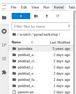
Open the launcher (the big blue + button) and open a new “Python 3” notebook.

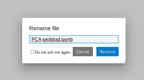
First things first, rename your new notebook to give it a meaningful name. You can either click the small ‘disk’ icon in the upper left corner of the notebook or choose File->Save Notebook

Import ipyrad.analysis module

The import keyword directs python to load a module into the currently running context. This is very similar to the library() function in R. We begin by importing the ipyrad analysis module. Copy the code below into a notebook cell and click run.

from ipyrad2.analysis.methods.pca import PCA

Quick guide (tl;dr)

The following cell shows the quickest way to results using the small simulated dataset in /scratch/ipyrad-workshop. Complete explanation of all of the features and options of the PCA module is the focus of the rest of this tutorial. Copy this code into a new notebook cell (small grey + button on the toolbar) and run it.

## Create the pca object with the simulated hdf5 data
pca = PCA.run(data="peddrad_outfiles/peddrad.hdf5")
## Bam!
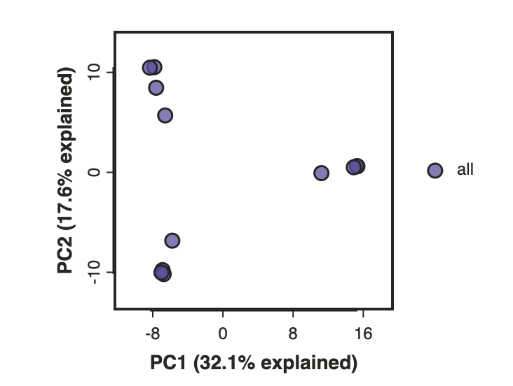
pca.draw()

Note: In this block of code, the # at the beginning of a line indicates to python that this is a comment, so it doesn’t try to run this line. This is a very handy thing if you want to add or remove lines of code from an analysis without deleting them. Simply comment them out with the #!

Full guide

Simple PCA from ipyrad hdf5 file

In the most common use, you’ll want to plot the first two PCs, then inspect the output, remove any obvious outliers, and then redo the PCA.

## Path to the input data in snps.hdf5 format 
data = "peddrad_outfiles/peddrad.hdf5"
pca = PCA(data)

Note: Here we use the hdf5 database file generated with ipyrad from the simulated data. The database file contains the genotype calls information as well as linkage information that is used for subsampling unlinked SNPs and bootstrap resampling.

Note: The ipyrad.analysis.pca module can also read in data from any vcf file, so it’s possible to quickly generate PCA plots for any vcf from any dataset.

Now construct the default plot, which shows all samples and PCs 1 and 2. By default all samples are assigned to one population, so everything will be the same color.

pca.draw()

Population assignment for sample colors

Typically it is useful to color points in a PCA by some a priori grouping, such as presumed population, or by experimental treatment groups, etc. this it is possible to specify population assignments in a text file. Sample names need to be identical to the names in the input dataset, which we can verify with the samples property of the PCA object. Open a new cell and type this:

pca.result.samples

['1A_0',
 '1B_0',
 '1C_0',
 '1D_0',
 '2E_0',
 '2F_0',
 '2G_0',
 '2H_0',
 '3I_0',
 '3J_0',
 '3K_0',
 '3L_0']

In the file browser on the left, left-click and create a new empty text file by choosing “New File”. The format of the population assignment file (or pops file) is a simple two column and whitespace separated (can be spaces or tabs). The first column is sample ID (must be identical to the results of pca.results.samples and the second column is Population. To save time, the first population looks like this. Copy this into your new file and finish filling out the rest of the population assignments for samples 2E_0 through 3L_0 (the populations they belong to are keyed by the first integer index of the sample ID).

1A_0 pop1
1B_0      pop1
1C_0    pop1
1D_0    pop1

When you are done click File->Save As and save this as sim_pops.txt. Now create the pca object with the input data again, this time passing in the new file name as the second argument and specifying this as the imap, and plot the new figure. We can also easily add a title to our PCA plots with the label= argument.

pca = PCA.run(data=data, imap="sim_pops.txt")
pca.draw(label="Sims colored by pop")

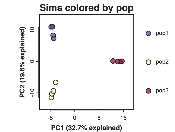
This is just much nicer looking now, and it’s also much more straightforward to interpret.

Evaluating applied filters and sample quality

It’s always important to keep an eye on the quality and completeness of your dataset during both the assembly and analysis steps. In particular missing data can cause weird patterns in PCA (with samples clustering by missingness rather than by meaningful biological variation) so it’s good to check for samples with excess missing data to potentially remove them.

You can ask PCA for a sample summary to check missingness stats:

pca.sample_summary()

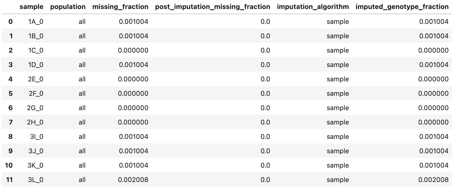
You can also inspect pre- and post-filtering stats to see the effect of each applied filter. This can be useful for tuning mincov/minmap filters to achieve a balance between reducing missing data and retaining enough SNPs to be informative.

pca.filter_summary()

samples                                        12.000
pre_filter_snps                              9425.000
pre_filter_percent_missing                      0.057
masked_genotypes_by_min_depth                   0.000
filter_by_indels_present                        0.000
filter_by_non_biallelic                       169.000
filter_by_mincov                                0.000
filter_by_minmap                                0.000
filter_by_min_site_qual                         0.000
filter_by_invariant_after_subsampling           0.000
filter_by_minor_allele_frequency                0.000
post_filter_snps                             9256.000
post_filter_snp_containing_linkage_blocks     996.000
post_filter_percent_missing                     0.058

Removing “bad” samples and replotting.

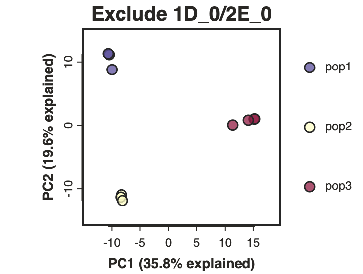
In PC analysis, it’s common for “bad” samples to dominate several of the first PCs, and thus “pop out” in a degenerate looking way. Bad samples of this kind can often be attributed to poor sequence quality or sample misidentifcation. Samples with lots of missing data tend to pop way out on their own, causing distortion in the signal in the PCs. Normally it’s best to evaluate the quality of the sample, and if it can be seen to be of poor quality, to remove it and replot the PCA. The simulated dataset is actually relatively nice, but for the sake of demonstration lets imagine the sample “1D_0” is ‘bad’.

Hover points in the PCA plot: We make a lot of use of the interactivity of jupyter notebooks in the ipyrad.analysis tools. In the PCA you can ‘hover’ over points to reveal their sample ID.

The easiest way to achieve this is to use the exclude parameter when calling PCA.run() to remove samples before running the PCA. This parameter takes a list of sample names (which is a comma separated group of strings enclosed in square brackets). Use it to exclude two samples like this:

pca = PCA.run(data=data, imap="sim_pops.txt", exclude=["1D_0", "2E_0"])
pca.draw(label="Exclude two samples")

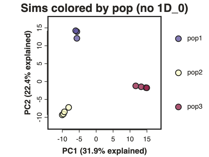
If you have many samples to exclude it might be easiert to simply remove these from the imap file and run the PCA again. Go to your sim_pops.txt file and remove “1D_0” then choose File->Save Text As and save this new pops file as subset_pops.txt.

pca = PCA.run(data=data, imap="subset_pops.txt")
pca.draw(label="Sims colored by pop (no 1D_0)")

Subsampling with replication

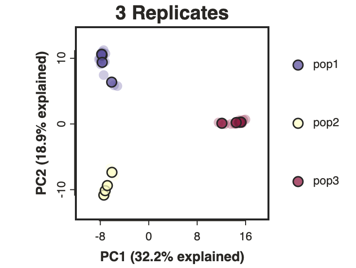
By default run() will randomly subsample one SNP per RAD locus to reduce the effect of linkage on your results. This can be turned off by setting subsample=False. However, subsampling unlinked SNPs is generally a good idea for PCA analyses since you want to remove the effects of linkage from your data. It also presents a convenient way to explore the confidence in your results. By using the option replicates you can run many replicate analyses that subsample a different random set of unlinked SNPs each time. The replicate results are drawn with a lower opacity and the centroid of all the points for each sample is plotted as a black point.

pca = PCA.run(data=data, imap="sim_pops.txt", replicates=25)
pca.draw(label="3 Replicates");

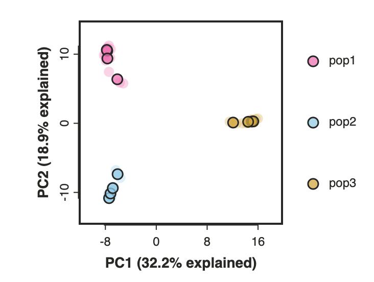
Custom color points

Another nice feature of the draw method is the ability to pass in any custom color that you like for each population. You can do this by passing in another tsv file this time mapping population IDs to python colors (either hexadecimal or named colors). The most straightforward is just to pass in a list of valid color names from the ‘named colors’ matplotlib documentation.

Open a new text file and save this as pop_colors.txt:

pop1	hotpink
pop2	skyblue
pop3	goldenrod

pca.draw(colors='pop_colors.txt')

Data imputation: Dealing with missing data in PCA

All PCA-family methods in ipyrad2 require a fully imputed genotype matrix. Missing genotypes are not allowed to remain in the numerical matrix passed to PCA, t-SNE, or UMAP.

Supported imputation modes are:

• sample: sample missing diploid genotypes from allele frequencies within each imputation group
• zero-fill: replace missing genotypes with homozygous reference calls

sample is the default and generally the preferred choice. If you provide imap, sample-mode imputation uses those groups. If you do not provide imap, all retained samples are treated as one imputation group.

zero-fill is usually a poor default for exploratory structure analyses because it can pull missing-heavy samples toward the reference state. Since none currently behaves the same way, users should not treat it as “leave missing data unchanged.”

Users should inspect sample_data_summary.tsv after every run and consider dropping samples that require too much imputation before trusting the structure. Heavy imputation is often a warning that missingness, rather than biology, may be shaping the ordination.

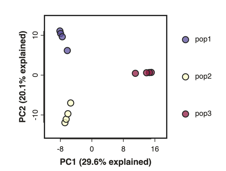
Here is an example of how to select the zero-fill impute_method (for the simulated data the results don’t change much):

pca = PCA.run(data=data, imap='sim_pops.txt', impute_method='zero-fill')
pca.draw()

Filtering data

Another approach is to simply enforce a lower bound on missing data with the min_sample_coverage parameter. This parameter specifies the minimum coverage threshold below which a snp is excluded from the analysis.

This code will exclude any snp not present in 100% of samples, a very strict threshold. Here we print the INFO again, so we can see how many SNPs were removed by this minimum sample coverage threshold.

pca = PCA.run(data=data, min_sample_coverage=12, log_level="INFO")

SNP extraction summary
  filter statistic samples: 12
  filter statistic pre_filter_snps: 9425
  filter statistic pre_filter_percent_missing: 0.057 (linked genotype cells missing before site filtering)
  filter statistic masked_genotypes_by_min_depth: 0
  filter statistic filter_by_indels_present: 0
  filter statistic filter_by_non_biallelic: 169
  filter statistic filter_by_mincov: 61
  filter statistic filter_by_minmap: 0
  filter statistic filter_by_min_site_qual: 0
  filter statistic filter_by_invariant_after_subsampling: 0
  filter statistic filter_by_minor_allele_frequency: 0
  filter statistic post_filter_snps: 9196
  filter statistic post_filter_snp_containing_linkage_blocks: 989

The INFO log level shows detailed information about all the filters that are applied prior to running the PCA. Some of these are required (indels, biallelic, invariant after subsampling), but others can also be controlled by parameters like min_minor_allele_frequency (MAF filters are common) and max_sample_missing (removing samples that exceed a given missingness threshold).

We encourage you to experiment with different imputation schemes and missing data thresholds when analysing your own data later.

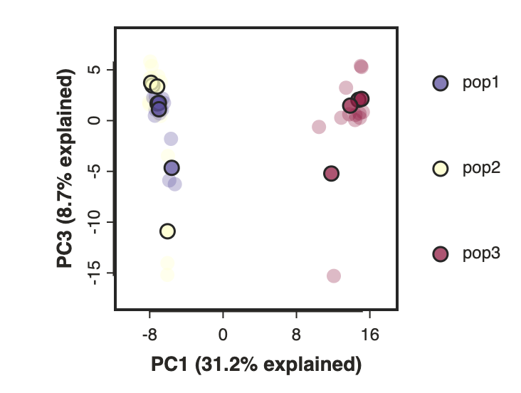
Plotting PCs other than the first and second

Even though PC 1 and 2 by definition explain the most variance in the data, it is still often useful to examine other PCs. You can do this by specifying which PCs to plot in in the call to draw.

• PC values are 0-indexed: We call it “PC 1” but because python is a zero-indexed for lists/arrays the first column of a matrix has index 0. We know it is confusing, and it is not just for you.

pca = PCA.run(data, imap="sim_pops.txt", replicates=3)
pca.draw(PC0=0, PC1=2)

Running ipyrad2 PCI CLI tool

The PCA notebook API tool we have been using is really just a wrapper around the command line version of the tool. The API mode makes it a bit easier to explore different plotting methods, but the underlying CLI tool has many more features that we don’t expose in the API.

$ ipyrad2 pca -h

usage: ipyrad2 pca -d Path [-n str] [-o Path] [-M str] [--replicates int] [--no-subsample] [--seed int] [--perplexity float]
                   [--max-iter int] [--n-neighbors int] [--plot] [--plot-width int] [--plot-height int] [--plot-marker-size int]
                   [--plot-colors Path] [-m int] [-r float] [-a float] [--min-genotype-depth int] [--min-site-qual float] [-I str]
                   [-e [str ...]] [-R] [-i Path] [-g Path] [-c int] [-f] [-l str] [-h]

-------------------------------------------------------------
ipyrad2 [v.0.1.11]
Interactive assembly and analysis of RAD-seq data
-------------------------------------------------------------
ipyrad2 pca: run PCA, t-SNE, or UMAP on SNP HDF5 data

Core inputs:
  -d, --data Path                         Path to an SNP-capable HDF5 file. Convert VCF first with `ipyrad2 vcf2hdf5`.
  -n, --name str                          Prefix name for output files. [default=pca]
  -o, --out Path                          Directory to write numerical outputs and stats. [default=output-pca]

Method and linkage:
  -M, --method str                        Method to run: pca, tsne, or umap. [default=pca]
  --replicates int                        Number of PCA replicate runs. Only valid with `-M pca`. [default=1]
  --no-subsample                          Keep linked SNPs. By default pca subsamples one SNP per RAD locus.
  --seed int                              Random seed for SNP subsampling, imputation, and serial method initialization.
  --perplexity float                      t-SNE perplexity. Used only with `-M tsne`. [default=5.0]
  --max-iter int                          t-SNE maximum iterations. Used only with `-M tsne`. [default=1000]
  --n-neighbors int                       UMAP neighbor count. Used only with `-M umap`. [default=15]

Plotting:
  --plot                                  Write an SVG plot for PCA results. Only supported with `-M pca`.
  --plot-width int                        SVG width in pixels for `--plot`. [default=400]
  --plot-height int                       SVG height in pixels for `--plot`. [default=300]
  --plot-marker-size int                  Marker size for `--plot`. [default=10]
  --plot-colors Path                      Whitespace-delimited population color file for PCA plot marker colors.

Filtering and samples:
  -m, --min-sample-coverage int           Minimum number of samples that must have data at a SNP. [default=4]
  -r, --max-sample-missing float          Maximum missing-data frequency allowed in a sample. [default=1.0]
  -a, --min-minor-allele-frequency float  Minimum minor allele frequency required to retain a SNP. [default=0.0]
  --min-genotype-depth int                Mask sample genotypes with FORMAT/DP below this threshold before site filtering. [default=0]
  --min-site-qual float                   Minimum VCF QUAL score required to retain a SNP site. [default=0.0]
  -I, --impute-method str                 Impute missing genotypes with `sample` or `zero`. [default=sample]
  -e, --exclude [str ...]                 Exclude one or more samples by name. This takes precedence over IMAP membership and `-R`.
  -R, --include-reference                 Include `assembly_reference_sequence`. By default it is excluded unless IMAP already contains it.
  -i, --imap Path                         Sample-to-population mapping file w/ `sample<TAB>population` or `glob<TAB>population` per line.
  -g, --minmap Path                       Population-to-minimum-coverage mapping file with `population<TAB>min` on each line. Adds per-
                                          population minimum coverage checks on top of `-m` when `imap` is used.

Performance and overwrite:
  -c, --cores int                         Number of cores to use during chunked SNP filtering and UMAP embedding. [default=1]
  -f, --force                             Overwrite existing output files with identical names.

Logging:
  -l, --log-level str                     Log level (TRACE, DEBUG, INFO, WARNING, ERROR) [default=INFO]
  -h, --help                              Show this help message and exit.

Examples
--------
$ ipyrad2 pca -d snps.hdf5 -o OUT/
$ ipyrad2 pca -d snps.hdf5 -o OUT/ --plot
$ ipyrad2 pca -d snps.hdf5 -o OUT/ --plot --plot-width 520 --plot-height 360
$ ipyrad2 pca -d snps.hdf5 -o OUT/ --plot -i imap.tsv --plot-colors colors.tsv
$ ipyrad2 pca -d snps.hdf5 -o OUT/ -M tsne --perplexity 8
$ ipyrad2 pca -d snps.hdf5 -o OUT/ -M umap --n-neighbors 10
$ ipyrad2 pca -d snps.hdf5 -o OUT/ --no-subsample --impute-method zero

More to explore

The ipyrad.analysis.methods.pca module has many more features that we just don’t have time to go over, but you might be interested in checking them out later:

• Full ipyrad PCA documentation