Setting up the environment and basic quality control

Before we get going with our first RAD-seq assembly, we need to get set up and oriented to our working environment. We make no assumptions about prior experience with cluster environments, so we scaffold the entire participant workshop experience from first principles. More advanced users hopefully will find value in some of the finer details we present.

Basic quality control (FastQC)
Viewing and interpreting FastQC results

Tutorial documentation conventions

Each grey cell in this tutorial indicates a command line interaction. Lines starting with $ indicate a command that should be executed in a terminal, for example by copying and pasting the text into your terminal. All lines in code cells beginning with ## are comments and should not be copied and executed. Elements in code cells surrounded by angle brackets (e.g. <username>) are variables that need to be replaced by the user. All other lines should be interpreted as output from the issued commands.

## Example Code Cell.
## Create an empty file in my home directory called `watdo.txt`
$ touch ~/watdo.txt

## Print "wat" to the screen
$ echo "wat"
wat

Examine the raw data

For this workshop we will be looking at and working with only the simulated data.

$ ls ipsimdata
gbs_example_barcodes.txt         pairddrad_example_genome.fa.smi        pairgbs_example_barcodes.txt         rad_example_barcodes.txt
gbs_example_genome.fa            pairddrad_example_R1_.fastq.gz         pairgbs_example_R1_.fastq.gz         rad_example_genome.fa
gbs_example_R1_.fastq.gz         pairddrad_example_R2_.fastq.gz         pairgbs_example_R2_.fastq.gz         rad_example_genome.fa.fai
pairddrad_example_barcodes.txt   pairddrad_wmerge_example_barcodes.txt  pairgbs_wmerge_example_barcodes.txt  rad_example_genome.fa.sma
pairddrad_example_genome.fa      pairddrad_wmerge_example_genome.fa     pairgbs_wmerge_example_genome.fa     rad_example_genome.fa.smi
pairddrad_example_genome.fa.fai  pairddrad_wmerge_example_R1_.fastq.gz  pairgbs_wmerge_example_R1_.fastq.gz  rad_example_R1_.fastq.gz
pairddrad_example_genome.fa.sma  pairddrad_wmerge_example_R2_.fastq.gz  pairgbs_wmerge_example_R2_.fastq.gz

Inspect the data

Then we will use the zcat command to read lines of data from one of the files and we will trim this to print only the first 20 lines by piping the output to the head command. Using a pipe (|) like this passes the output from one command to another and is a common trick in the command line.

Here we have our first look at a fastq formatted file. Each sequenced read is spread over four lines, one of which contains sequence and another the quality scores stored as ASCII characters. The other two lines are used as headers to store information about the read.

$ zcat ipsimdata/rad_example_R1_.fastq.gz | head -n 20
@lane1_locus0_2G_0_0 1:N:0:
CTCCAATCCTGCAGTTTAACTGTTCAAGTTGGCAAGATCAAGTCGTCCCTAGCCCCCGCGTCCGTTTTTACCTGGTCGCGGTCCCGACCCAGCTGCCCCC
+
BBBBBBBBBBBBBBBBBBBBBBBBBBBBBBBBBBBBBBBBBBBBBBBBBBBBBBBBBBBBBBBBBBBBBBBBBBBBBBBBBBBBBBBBBBBBBBBBBBBB
@lane1_locus0_2G_0_1 1:N:0:
CTCCAATCCTGCAGTTTAACTGTTCAAGTTGGCAAGATCAAGTCGTCCCTAGCCCCCGCGTCCGTTTTTACCTGGTCGCGGTCCCCACCCAGCTGCCCCC
+
BBBBBBBBBBBBBBBBBBBBBBBBBBBBBBBBBBBBBBBBBBBBBBBBBBBBBBBBBBBBBBBBBBBBBBBBBBBBBBBBBBBBBBBBBBBBBBBBBBBB
@lane1_locus0_2G_0_2 1:N:0:
CTCCAATCCTGCAGTTTAACTGTTCAAGTTGGCAAGATCAAGTCGTCCCTAGCCCCCGCGTCCGTTTTTACCTGGTCGCGGTCCCGACCCAGCTGCCCCC
+
BBBBBBBBBBBBBBBBBBBBBBBBBBBBBBBBBBBBBBBBBBBBBBBBBBBBBBBBBBBBBBBBBBBBBBBBBBBBBBBBBBBBBBBBBBBBBBBBBBBB
@lane1_locus0_2G_0_3 1:N:0:
CTCCAATCCTGCAGTTTAACTGTTCAAGTTGGCAAGATCAAGTCGTCCCTAGCCCCCGCGTCCGTTTTTACCTGGTCGCGGTCCCGACCCAGCTGCCCCC
+
BBBBBBBBBBBBBBBBBBBBBBBBBBBBBBBBBBBBBBBBBBBBBBBBBBBBBBBBBBBBBBBBBBBBBBBBBBBBBBBBBBBBBBBBBBBBBBBBBBBB
@lane1_locus0_2G_0_4 1:N:0:
CTCCAATCCTGCAGTTTAACTGTTCAAGTTGGCAAGATCAAGTCGTCCCTAGCCCCCGCGTCCGTTTTTACCTGGTCGCGGTCCCGACCCAGCTGCCCCC
+
BBBBBBBBBBBBBBBBBBBBBBBBBBBBBBBBBBBBBBBBBBBBBBBBBBBBBBBBBBBBBBBBBBBBBBBBBBBBBBBBBBBBBBBBBBBBBBBBBBBB

Here the quality scores are all uniformly high (probability of miscalled base < 0.0005), because it’s simulated. The fastqc wikipedia page actually has a really nice section on quality score interpretation. Real data will look more like this:

@HWI-D00289:107:C3J97ACXX:6:1101:1420:2169 1:N:0:CGTACG
CGAATCATGCATTATTTATTTATGTATTACATTTGTATAGTGCTCTAACCCTCAGGCATCTGAGCGCTTCTTACATGGTTACATTTAGTTACATTGGTTGC
+
BB<BBBFBBB0<F<0<BBBFB<FF<<BBFBBBFBF<BF<BB<7B0B70BFFFFFFBF0BFBFBBBFIBBBBBFFB<<BBB7<<BB<<<BF7<<BBBBBBBB
@HWI-D00289:107:C3J97ACXX:6:1101:1737:2150 1:N:0:CGTACG
ACTTCCATGCTCACAGTGAAATCAGTGCTGGACATCGTGGGTCCAAGAAAACGGCCGAGATATTGATGGAAGTGGCTTACTGGCCGCATCTATATCAAGAT
+
B<BFFF<B0BFBFFFIBBFBIFIIFB0BBFFFFBFFFBFF7BFBBB7BFFB'BBFBFFF<FFFFF<BBBBBBBBBBBBBBBBBBBBBBBB<'<<BBBBB<B
@HWI-D00289:107:C3J97ACXX:6:1101:1806:2113 1:N:0:CGTACG
ACTGGCATGCTGACAATATGCACATGGATGATGACACACTACGATACTGGCATGTGAATGGAATATTGGGTGAGGGGCAACCACAATGCAATACTGTTGTA
+
BBBFFFFFFFFFFIIIIIIIIIIIIIIIIIIIFFIIIIIIIIFIIIIIIIIIIFFIBFFIIFIIIFFBFIBFFFFFFFBBFFFFBFBBFFFFFFFFFFBBF
@HWI-D00289:107:C3J97ACXX:6:1101:1809:2136 1:N:0:CGTACG
ATTACAAGAAGGGACTCTGTCCCTGATTGGGAGCATATATTGAAGTGATCGTGATCTCCGTAAGCTTAATTCTGCCTTTTACTATAATGTACCTTCCCTTC
+
BBBFFBFFFFFFFF7FFF<BFFIFF0<B7BF'BFBBBBFFBFBFF7BBFFFFF7BBBFFF7FBFFFI'<BFFFFFF<BBF<BB0<BBBBBBBBB7'77<BB

FastQC for quality control

The first step of any RAD-Seq assembly is to inspect your raw data to estimate overall quality. We began first with a visual inspection above, but of course we can only visually inspect a very tiny proportion of the total data. So instead we use automated approaches to check the quality of our data.

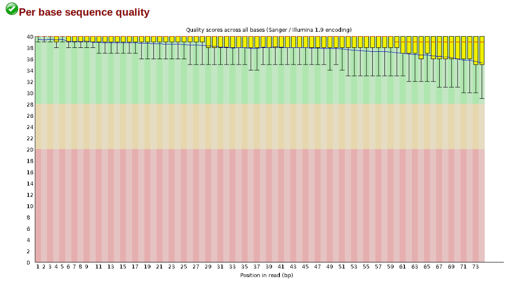
At this stage you can then attempt to improve your dataset by identifying and removing samples with failed sequencing. Another key QC procedure involves inspecting average quality scores per base position and trimming read edges, which is where low quality base-calls tend to accumulate. In this figure, the X-axis shows the position on the read in base-pairs and the Y-axis depicts information about Phred quality score per base for all reads, including median (center red line), IQR (yellow box), and 10%-90% (whiskers). As an example, here is a very clean base sequence quality report for a 75bp RAD-Seq library. These reads have generally high quality across their entire length, with only a slight (barely worth mentioning) dip toward the end of the reads:

png

In contrast, here is a somewhat typical base sequence quality report for R1 of a 300bp paired-end Illumina run of ezrad data:

png

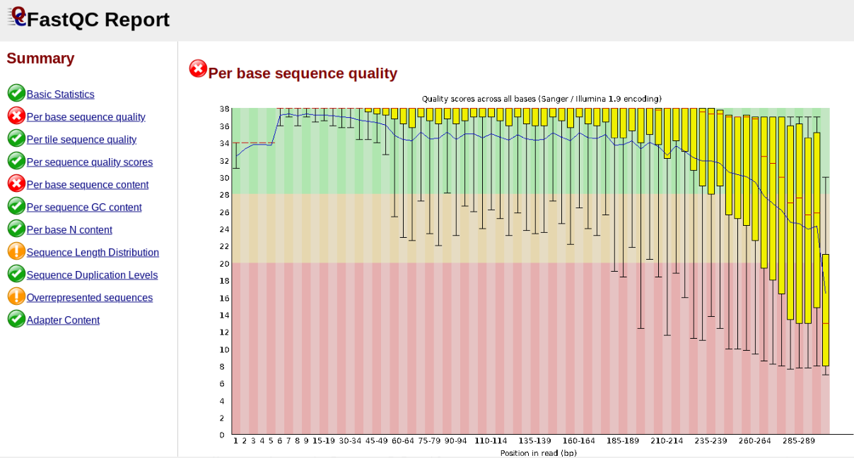
This figure depicts a common artifact of current Illumina chemistry, whereby quality scores per base drop off precipitously toward the ends of reads, with the effect being magnified for read lengths > 150bp. The purpose of using FastQC to examine reads is to determine whether and how much to trim our reads to reduce sequencing error interfering with basecalling. In the above figure, as in most real dataset, we can see there is a tradeoff between throwing out data to increase overall quality by trimming for shorter length, and retaining data to increase value obtained from sequencing with the result of increasing noise toward the ends of reads.

Running FastQC

In the interest of saving time during this short workshop we will only indicate how fastqc is run, and will then focus on interpretation of typical output. More detailed information about actually running fastqc are available elsewhere on the RADCamp site.

For future reference, you can install fastqc from the bioconda channel:

$ conda install -c bioconda fastqc -y

NB: The -y here just tells conda “When you ask if I’m sure I want to install, the answer is YES!”, prevents it from prompting you.

To run fastqc on one of the simulated samples you may execute this command:

$ mkdir fastqc-results

# The -o flag tells fastqc where to write output files.
$ fastqc -o fastqc-results ipsimdata/rad_example_R1_.fastq.gz

Note: Running fastqc on real data can be somewhat slow, plus most of the samples from one library should look mostly the same. It is always good practice to actually look at your data before proceeding with the assembly, but you don’t have to look at all of it. Typically 3-5 randomly selected samples should give a good overall view of quality.

Inspecting and Interpreting FastQC Output

Simulated data is too clean to be interesting, so lets spend a moment looking at the results from some real data from Prates et al (2016) (Anolis punctatus, GBS data).

png

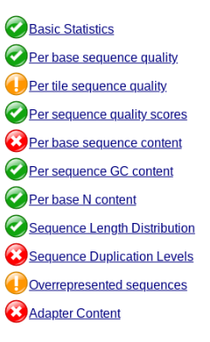
Lets start with Per base sequence quality, because it’s very easy to interpret, and often times with RAD-Seq data results here will be of special importance.

png

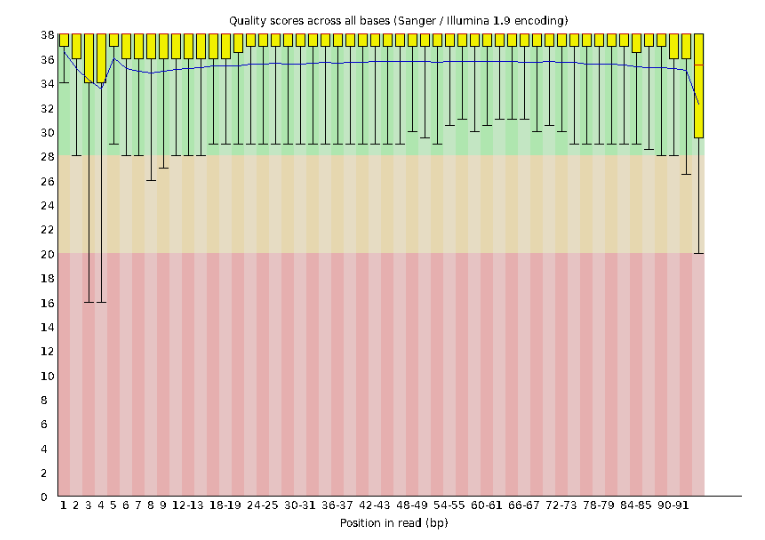
For the Anolis data the sequence quality per base is uniformly quite high, with dips only in the first and last 5 bases (again this is typical for Illumina reads). Based on information from this plot we can see that the Anolis data doesn’t need a whole lot of trimming, which is good.

Now lets look at the Per base sequece content, which FastQC highlights with a scary red X. png

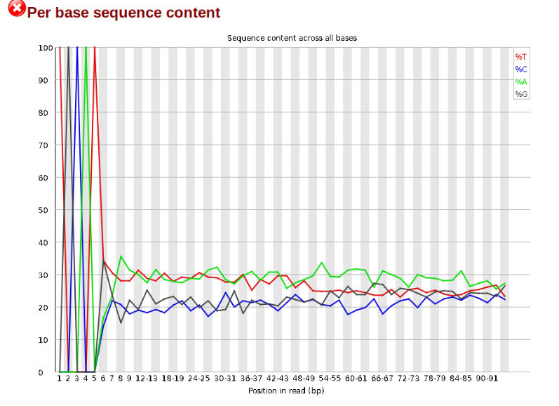
The squiggles indicate base composition per base position averaged across the reads. It looks like the signal FastQC is concerned about here is related to the extreme base composition bias of the first 5 positions. We happen to know this is a result of the restriction enzyme overhang present in all reads (TGCAT in this case for the EcoT22I enzyme used), and so it is in fact of no concern. Now lets look at Adapter Content:

png

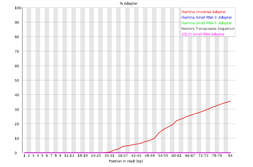
Here we can see adapter contamination increases toward the tail of the reads, approaching 40% of total read content at the very end. The concern here is that if adapters represent some significant fraction of the read pool, then they will be treated as “real” data, and potentially bias downstream analysis. In the Anolis data this looks like it might be a real concern so if we were assembling this dataset we’d want to keep this in mind during step 2 of the ipyrad analysis, and incorporate 3’ read trimming and aggressive adapter filtering.

Other than this, the data look good and we can proceed with the ipyrad analysis.

References

Prates, I., Xue, A. T., Brown, J. L., Alvarado-Serrano, D. F., Rodrigues, M. T., Hickerson, M. J., & Carnaval, A. C. (2016). Inferring responses to climate dynamics from historical demography in neotropical forest lizards. Proceedings of the National Academy of Sciences, 113(29), 7978-7985.