The ipyrad.analysis module: Parallelized STRUCTURE analyses on unlinked SNPs
As part of the ipyrad.analysis toolkit we’ve created convenience functions for easily distributing STRUCTURE analysis jobs on an HPC cluster, and for doing so in a programmatic and reproducible way. Importantly, our workflow allows you to easily sample different distributions of unlinked SNPs among replicate analyses, with the final inferred population structure summarized from a distribution of replicates. We also provide some simple examples of interactive plotting functions to make barplots.
Why STRUCTURE?
Although there are many newer and faster implementations of STRUCTURE, such as faststructure or admixture, the original STRUCTURE works much better with missing data, which is of course a common feature of RAD-seq data sets.
What is the “true” value of K?
Identifying the true number of genetic clusters in a sample is a long standing, and difficult problem (see for example Evanno et al 2005, Verity & Nichols 2016, and partiulcarly Janes et al 2017 (titled “The K = 2 conundrum”). Famously, the method of identifying the best K presented in Pritchard et al (2000) is described as “dubious at best”. Even Evanno et al (2005) (cited over 12,000 times) “… insist that this (deltaK) criterion is another ad hoc criterion….” Because of this we stress that population structure analysis is as an exploratory method, and should be approached in a heirarchical fashion.
STRUCTURE Analyses
Configure HPC environment for ipyparallel (THIS IS VERY IMPORTANT)
In this tutorial we will be using a python package for parallel computation called ipyparallel. The USP cluster does not have a GUI, as is typical of cluster systems. Unfortunately ipyparallel and this particular GUI-less environment have a hard time interacting (for complicated reasons). We have derived a workaround that allows the parallelization to function. You should execute the following commands in a terminal on the USP cluster before doing anything else.
VERY IMPORTANT: This environment variable needs to be set in both .bashrc and .profile so that it is picked up when you run ipyparallel in either the head node of the cluster or on compute nodes.
$ echo "# Prevent ipyparallel engines from dying in a headless environment" >> ~/.bashrc
$ echo "export QT_QPA_PLATFORM=offscreen" >> ~/.bashrc
$ echo "export QT_QPA_PLATFORM=offscreen" >> ~/.profile
$ source ~/.bashrc
$ source ~/.profile
$ env | grep QT
QT_QPA_PLATFORM=offscreen
Note: Don’t worry if this seems like black magic, because IT IS! ;p
First, begin by creating a new notebook inside your /home/<username>/ipyrad-workshop/ directory called anolis-structure.ipynb (refer to the jupyter notebook configuration page for a refresher on connecting to the notebook server). The rest of the materials in this part of the workshop assume you are running all code in cells of a jupyter notebook that is running on the USP cluster.
Required software
You can easily install the required software for this notebook using conda. This can even be accomplished inside your jupyter notebook. Preceding a command with ! will tell the notebook to run the line as a terminal command, instead of as python.
## The `-y` here means "Answer yes to all questions". It prevents
## conda from asking whether the install looks ok.

!conda install -y -c ipyrad structure clumpp
Solving environment: done
## Package Plan ##
...
...
Preparing transaction: done
Verifying transaction: done
Executing transaction: done
Note: You only have to run this conda install command once on the cluster. It does not need to be run every time you run a notebook or every time you create a new notebook. Once the install finishes STRUCTURE and CLUMPP will be available for all your notebooks.
Import Python libraries
import ipyrad.analysis as ipa   ## ipyrad analysis toolkit
import ipyparallel as ipp       ## parallel processing
import toyplot                  ## plotting library
Parallel cluster setup
Normally, Jupyter notebook processes run on just one core. If we want to run multiple iterations of an algorithm then we would have to run them one at a time, and this is tedious and time consuming. Fortunately, Jupyter notebook servers have a built in parallelization engine (ipcluster), which is really easy to use.
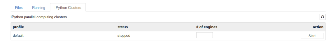
A very easy way to start the ipcluster parallelization backend is to go to your Jupyter dashboard, choose the IPython Clusters tab, choose the number of “engines” (the number of independent processes), and click Start.
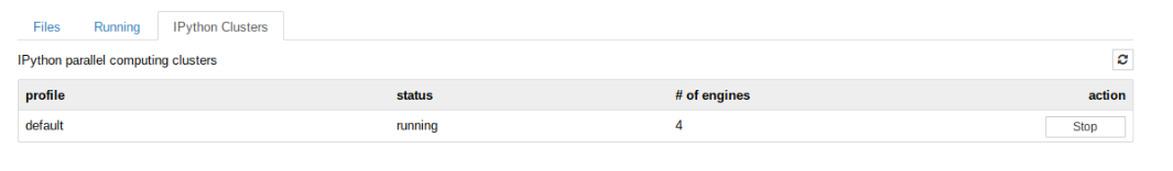
Now you have 4 mighty cores to process your jobs instead of just 1!
How do we interact with or ipcluster? Lets just get some information from it first:
## get parallel client
ipyclient = ipp.Client()
print("Connected to {} cores".format(len(ipyclient)))
Connected to 4 cores > **Note:** The `format()` function takes arguments and "formats" them properly for insertion into a string. In this case it takes the Integer value of `len(ipyclient)` (the count of the number of engines) and substitutes this in place of `{}` in the output.
Quick guide (tl;dr)
The following cell shows the quickest way to results. Detailed explanations of all of the features and options are provided further below.
## set N values of K to test across
kvalues = [2, 3, 4]

## init an analysis object
struct = ipa.structure(
    name="anolis-quick",
    workdir="./anolis-structure",
    data="./anolis_outfiles/anolis.ustr",
    )

## set main params (use much larger values in a real analysis)
struct.mainparams.burnin = 1000
struct.mainparams.numreps = 5000

## submit 5 replicates of each K value to run on parallel client
for kpop in kvalues:
    struct.run(kpop=kpop, nreps=5, ipyclient=ipyclient)

## wait for parallel jobs to finish
ipyclient.wait()
submitted 5 structure jobs [quick-K-2]
submitted 5 structure jobs [quick-K-3]
submitted 5 structure jobs [quick-K-4]

True
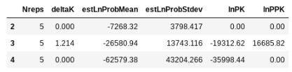
## return the evanno table (deltaK) for best K
etable = struct.get_evanno_table(kvalues)
etable
## get admixture proportion tables averaged across reps
tables = struct.get_clumpp_table(kvalues, quiet=True)
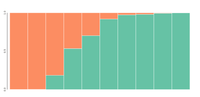
## bar plot for k=2, sorted by columns of the Q-matrix
table = tables[2].sort_values(by=[0, 1])

toyplot.bars(
    table,
    width=500,
    height=200,
    title=[[i] for i in table.index.tolist()],
    xshow=False,
);
Full guide
Enter input and output file locations
The .str file is a STRUCTURE formatted file output by ipyrad. It includes all SNPs present in the data set. The .snps.map file is an optional file that maps which locus each SNP is from. If this file is used then each replicate analysis will randomly sample a single SNP from each locus in reach rep. The results from many reps therefore will represent variation across unlinked SNP data sets, as well as variation caused by uncertainty. The .ustr file that was used in the tl;dr analysis represents just one sample of unlinked snps (i.e. one random snp per locus), so it’s good for quick and dirty analysis, but it doesn’t fully capture uncertainty in the data. The workdir is the location where you want output files to be written and will be created if it does not already exist.
NB: If you have the full .str. and the snps.map file it is generally better to use these to run multiple replictes, and then average over these replicates with CLUMPP. Here, we only use the .ustr file in the tl;dr example to illustrate the general workflow.
## the structure formatted file
strfile = "./anolis_outfiles/anolis.str"

## an optional mapfile, to sample unlinked SNPs
mapfile = "./anolis_outfiles/anolis.snps.map"

## the directory where outfiles should be written
workdir = "./anolis-structure/"
Note: The .str/.map file combination is more robust and more fully captures the variation in the data. The .ustr file is one sample of unlinked snps that’s useful for basic exploratory analysis.
Create a STRUCTURE Class object
STRUCTURE is kind of an old fashioned program that requires creating quite a few input files to run, which makes it not very convenient to use in a programmatic and reproducible way. To work around this the ipyrad.analysis.structure module introduces a convenience wrapper object to make it easy to submit STRUCTURE jobs and to summarize their results.
## create a Structure object
struct = ipa.structure(name="anolis-test",
                       data=strfile,
                       mapfile=mapfile,
                       workdir=workdir)
Set parameter options for this object
The STRUCTURE object will be used to submit jobs to the ipyparallel cluster. It has associated with it a name, a set of input files, and a large number of parameter settings. You can modify the parameters by setting them like below. You can also use tab-completion to see all of the available options, or print them like below. See the full STRUCTURE docs here for further details on the function of each parameter. In support of reproducibility, it’s good practice to print both the mainparams and extraparams so it’s clear which options you used.
## set mainparams for object
struct.mainparams.burnin = 1000
struct.mainparams.numreps = 5000

## see all mainparams
print struct.mainparams

## see or set extraparams
print struct.extraparams
burnin             10000
extracols          0
label              1
locdata            0
mapdistances       0
markernames        0
markovphase        0
missing            -9
notambiguous       -999
numreps            100000
onerowperind       0
phased             0
phaseinfo          0
phenotype          0
ploidy             2
popdata            0
popflag            0
recessivealleles   0

admburnin           500
alpha               1.0
alphamax            10.0
alphapriora         1.0
alphapriorb         2.0
alphapropsd         0.025
ancestdist          0
ancestpint          0.9
computeprob         1
echodata            0
fpriormean          0.01
fpriorsd            0.05
freqscorr           1
gensback            2
inferalpha          1
inferlambda         0
intermedsave        0
lambda_             1.0
linkage             0
locispop            0
locprior            0
locpriorinit        1.0
log10rmax           1.0
log10rmin           -4.0
log10rpropsd        0.1
log10rstart         -2.0
maxlocprior         20.0
metrofreq           10
migrprior           0.01
noadmix             0
numboxes            1000
onefst              0
pfrompopflagonly    0
popalphas           0
popspecificlambda   0
printlambda         1
printlikes          0
printnet            1
printqhat           0
printqsum           1
randomize           0
reporthitrate       0
seed                12345
sitebysite          0
startatpopinfo      0
unifprioralpha      1
updatefreq          10000
usepopinfo          0                    > **Note:** Don't worry about trying to understand all of these parameters at this time. The defaults are sensible. But do notice that the `burnin` and `numreps` here are still well below the values you'd use in real analysis, typically more on the order of 1 million for `numreps`.
Submit many jobs to run in parallel
The function run() distributes jobs to run on the cluster via the ipyparallel backend. It takes a number of arguments. The first, kpop, is the number of populations. The second, nreps, is the number of replicated runs to perform. Each rep has a different random seed, and if you entered a mapfile for your STRUCTURE object then it will subsample unlinked SNPs independently in each replicate. The seed argument can be used to make the replicate analyses reproducible (i.e. a STRUCTURE run using the same SNPs and started with the same seed will always produce the same results). The extraparams.seed parameter will be generated from this for each replicate. And finally, provide it the ipyclient object that we created above. The STRUCTURE object will store an asynchronous results object for each job that is submitted so that we can query whether the jobs are finished. Using a simple for-loop we’ll submit 10 replicate jobs to run at three different values of K.
## a range of K-values to test
kvalues = [2, 3, 4]

## submit batches of 10 replicate jobs for each value of K
for kpop in kvalues:
    struct.run(
        kpop=kpop,
        nreps=10,
        seed=12345,
        ipyclient=ipyclient,
        )
submitted 10 structure jobs [structure-test-K-2]
submitted 10 structure jobs [structure-test-K-3]
submitted 10 structure jobs [structure-test-K-4]
Note This step may take some time…
Track progress until finished
A straightforward way to monitor the progress of structure replicates is to just ask the jobs whether they are finished yet. The list of jobs for a STRUCTURE analysis are retained in the asysncs list, which is a list of the “asynchronous” responses we are awaiting from the structure tasks we created. They are “asynchronous” because they are independent and the runtimes are somewhat unknown. We can ask all of the jobs whether any of them are finished:
## check if a specific job is done
for async in struct.asyncs:
    print(async.ready()),
True True True True True True True True True True False False False False False False False False False False False False False False False False False False False False
The number of True values you see here indicates the number of replicates that are finished. You can keep running this last command this over and over again until all job returns True, but this is tedious. Simpler is to block/wait until all jobs are finished by using the wait() function of the ipyclient object:
## block/wait until all jobs finished
ipyclient.wait()
Returning from break
import ipyrad.analysis as ipa   ## ipyrad analysis toolkit
import ipyparallel as ipp       ## parallel processing
import toyplot                  ## plotting library

ipyclient = ipp.Client()
print(len(ipyclient))

strfile = "./anolis_outfiles/anolis.str"
mapfile = "./anolis_outfiles/anolis.snps.map"
workdir = "/scratch/af-biota/anolis-structure/"

struct = ipa.structure(name="anolis-structure",
                       data=strfile,
                       mapfile=mapfile,
                       workdir=workdir)
Summarize replicates with CLUMPP
We ran 10 replicates per K-value hypothesis. In order to summarize results across these replicates we use the software CLUMPP.
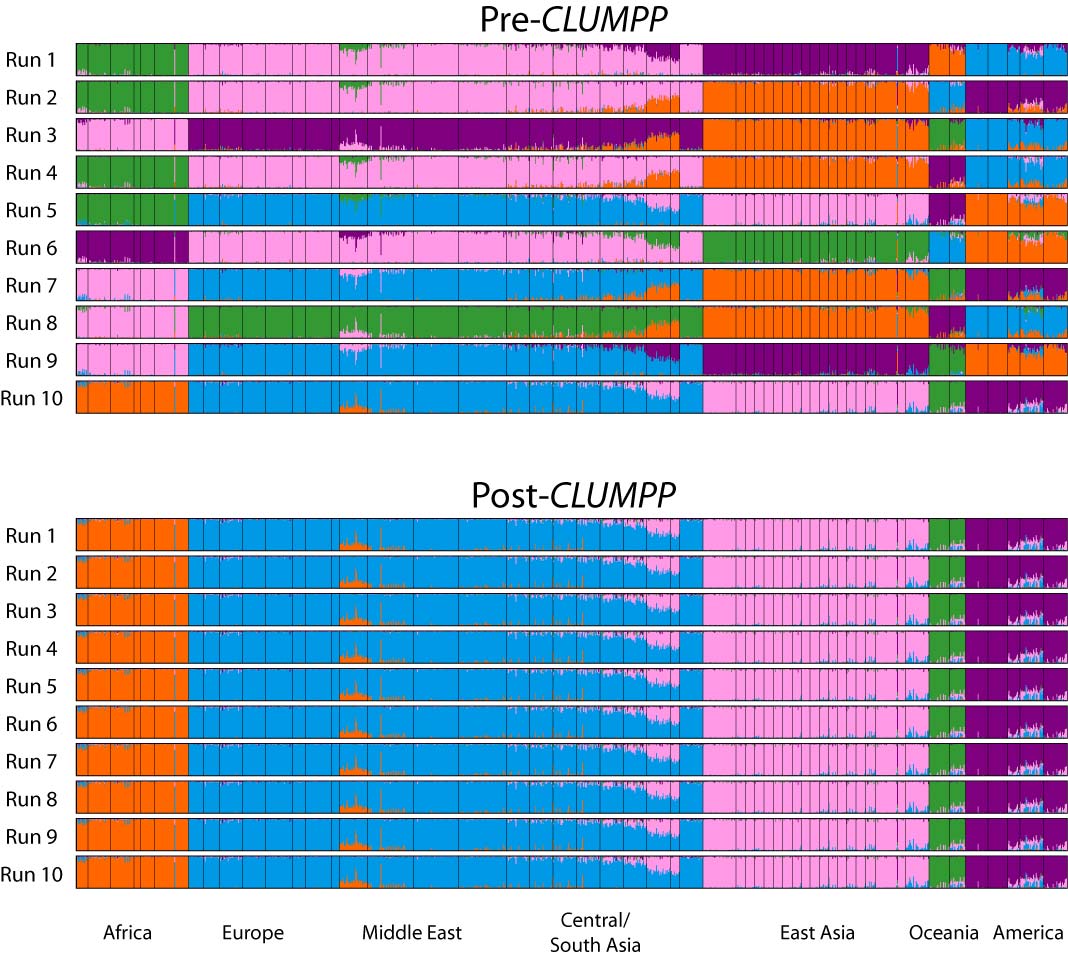
The default arguments to CLUMPP are generally good, but if you’re running a dataset with high numbers of K, you may want to modify the greedy_option, for example. However, we don’t need to do this with the dataset for this workshop. You can modify the parameters in the same as the STRUCTURE params, by accessing the .clumppparams attribute of your STRUCTURE object. See the CLUMPP documentation for more details. Below we run CLUMPP for each value of K that we ran STRUCTURE on. You only need to tell the get_clumpp_table() function the value of K and it will find all of the result files given the STRUCTURE object’s name and workdir.
## set some clumpp params and print params to the screen
struct.clumppparams.repeats = 10000
struct.clumppparams
datatype                  0
every_permfile            0
greedy_option             2
indfile                   0
m                         3
miscfile                  0
order_by_run              1
outfile                   0
override_warnings         0
permfile                  0
permutationsfile          0
permuted_datafile         0
popfile                   0
print_every_perm          0
print_permuted_data       0
print_random_inputorder   0
random_inputorderfile     0
repeats                   10000
s                         2
w                         1
## run clumpp for each value of K
tables = struct.get_clumpp_table(kvalues)
[K2] 10/10 results permuted across replicates (max_var=0).
[K3] 10/10 results permuted across replicates (max_var=0).
[K4] 10/10 results permuted across replicates (max_var=0).
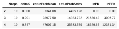
## return the evanno table w/ deltaK
struct.get_evanno_table(kvalues)
Sort the table order how you like it
This can be useful if, for example, you want to order the names to be in the same order as tips on your phylogeny.
## custom sorting order
myorder = [
    "punc_ICST764",
    "punc_MUFAL9635",
    "punc_IBSPCRIB0361",
    "punc_JFT773",
    "punc_MTR05978",
    "punc_MTR17744",
    "punc_MTR21545",
    "punc_MTR34414",
    "punc_MTRX1468",
    "punc_MTRX1478"
]
We can then extract the results for any give K value with the samples in the order that we want them. Here we inspect the ancestry components for K=3.
print("custom ordering")
print(tables[3].loc[myorder])
custom ordering
                       0          1      2
punc_ICST764       0.102  8.000e-04  0.897
punc_MUFAL9635     0.139  1.000e-03  0.860
punc_IBSPCRIB0361  0.021  9.774e-01  0.001
punc_JFT773        0.132  8.340e-01  0.034
punc_MTR05978      0.844  5.980e-02  0.097
punc_MTR17744      0.115  8.566e-01  0.029
punc_MTR21545      0.267  5.963e-01  0.137
punc_MTR34414      0.394  4.582e-01  0.148
punc_MTRX1468      0.028  9.590e-01  0.013
punc_MTRX1478      0.044  9.532e-01  0.002
Note: The
.loc[]notation specifies to fetch from the table by row.
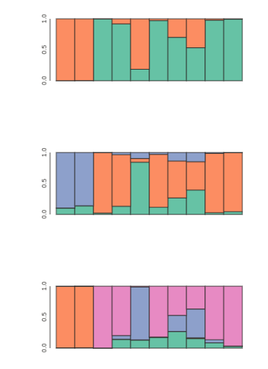
Visualize population STRUCTURE in barplots
for kpop in kvalues:
    ## parse outfile to a table and re-order it
    table = tables[kpop]
    table = table.ix[myorder]

    ## plot barplot w/ hover
    canvas, axes, mark = toyplot.bars(
                            table,
                            width=400,
                            height=200,
                            style={"stroke": toyplot.color.near_black},
                            )
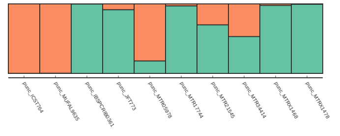
Make a slightly fancier plot and save to file
Lets define a function to make the fancy plot, so we can call the function multiple times easily. The def keyword indicates that we are “defining” a python function.
def fancy_plot(table):
    import toyplot
    ## further styling of plot with css
    style = {"stroke":toyplot.color.near_black,
         "stroke-width": 2}

    ## build barplot
    canvas = toyplot.Canvas(width=800, height=400)
    axes = canvas.cartesian(bounds=("5%", "95%", "5%", "45%"))
    axes.bars(table, style=style)

    ## add names to x-axis
    ticklabels = [i for i in table.index.tolist()]
    axes.x.ticks.locator = toyplot.locator.Explicit(labels=ticklabels)
    axes.x.ticks.labels.angle = -60
    axes.x.ticks.show = True
    axes.x.ticks.labels.offset = 10
    axes.x.ticks.labels.style = {"font-size": "12px"}
    axes.x.spine.style = style
    axes.y.show = False

    import toyplot.svg
    import toyplot.pdf
    toyplot.svg.render(canvas, "anolis-struct.svg")
    toyplot.pdf.render(canvas, "anolis-struct.pdf")

    ## show in notebook
    return canvas
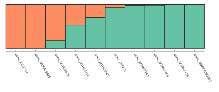
Now we can call our fancy_plot() function using the sample order we defined earlier and K=2.
## save plots for your favorite value of K
table = struct.get_clumpp_table(kvalues=2)
table = table.loc[myorder]
fancy_plot(table)
[K2] 10/10 results permuted across replicates (max_var=0).
Alternatively if we want to just sort by increasing values of ancestry components we can use the sort_values() function, which is illustrated below:
table = struct.get_clumpp_table(kpop=2)
table = table.sort_values(by=[0, 1])
fancy_plot(table)
Testing for convergence
The .get_evanno_table() and .get_clumpp_table() functions each take an optional argument called max_var_multiple, which is the max multiple by which you’ll allow the variance in a ‘replicate’ run to exceed the minimum variance among replicates for a specific test. In the example below you can see that many reps were excluded for the higher values of K, such that fewer reps were analyzed for the final results. By excluding the reps that had much higher variance than other (one criterion for asking if they converged) this can increase the support for higher K values. If you apply this, method take care to think about what it is doing and how to interpret the K values. Also take care to consider whether your replicates are using the same input SNP data but just different random seeds, or if you used a map file, in which case your replicates represent different sampled SNPs and different random seeds. I’m of the mind that there is no true K value, and sampling across a distribution of SNPs across many replicates gives you a better idea of the variance in population structure in your data.
struct.get_evanno_table([2, 3, 4], max_var_multiple=10.)
[K2] 2 reps excluded (not converged) see 'max_var_multiple'.
[K3] 7 reps excluded (not converged) see 'max_var_multiple'.
[K4] 5 reps excluded (not converged) see 'max_var_multiple'.