The ipyrad.analysis module: RAxML
As part of the ipyrad.analysis toolkit we’ve created convenience functions for easily running common RAxML commands, a maximum likelihood inference of phylogenetic trees. This can be useful when you want to run all of your analyses in a clean stream-lined way in a jupyter notebook to create a completely reproducible study.
Install software
There are many ways to install RAxML, the simplest of which is to use conda. This will install several RAxML binaries into your conda path. Open an ssh session on the cluster and run the following command:
$ conda install raxml -c bioconda
RAxML Phylogenetic Inference
Create a new notebook inside your /home/<username>/ipyrad-workshop/ directory called anolis-raxml.ipynb (refer to the jupyter notebook configuration page for a refresher on connecting to the notebook server). The rest of the materials in this part of the workshop assume you are running all code in cells of a jupyter notebook that is running on the USP cluster.
Create a RAxML Class object
First, copy and paste the usual imports into a notebook cell and run it:
import ipyrad.analysis as ipa    ## ipyrad analysis toolkit
import toyplot                   ## plotting library
import toytree                   ## tree plotting
Now create a RAxML object. The only required argument to initialize the object is a phylip formatted sequence file. In this example we provide a name and working directory as well:
rax = ipa.raxml(
    data="./anolis_outfiles/anolis.phy",
    name="anolis-tree",
    workdir="./anolis-raxml",
    );
Additional options
RAxML has a ton of parameters for modifying how it behaves, and we will only explore just a fraction of these. For more info on RAxML parameters, look here. You can also specify many of these parameters by setting values in the params dictionary of your RAxML object. In the following cell we modify the number of bootstrapping runs on distinct starting trees (params.N), the number of threads to use (params.T), and the outgroup samples (params.o).
## Number of runs
rax.params.N = 10

## Number of threads
rax.params.T = 2

## Set the outgroup. Because we don't have an outgroup for Anolis we use None.
rax.params.o = None

## Alternatively, if we had an outgroup we could specify this with sample names
## Here we could specify the Northern samples as the outgroup, this is just for illustration
## rax.params.o = ['punc_ICST764', 'punc_MUFAL9635']
Print the command string
It is good practice to always print the command string so that you know exactly what was called for your analysis and it is documented.
print(rax.command)
raxmlHPC-PTHREADS-SSE3 -f a -T 2 -m GTRGAMMA -N 10 -x 12345 -p 54321 -n anolis-tree -w /home/<username>/ipyrad-workshop/anolis-raxml -s /home/<username>/ipyrad-workshop/anolis_outfiles/anolis.phy
Explanation of RAxML arguments:
- -f: selects the algorithm RAxML will execute. In this case,
-f awill perform a rapid bootstrap analysis and search for best-scoring ML tree in a single run. - -T: specifies the number of threads you want to run. This should reflect the number of cores available in your machine, only 2 in our case.
- -m: selects the model of nucleotide substitution. In this case, GTRGAMMA is the GTR (generalised time-reversible) + GAMMA model of rate heterogeneity. A complex, but standard model used in RAxML.
- -N: specifies the number of alternative runs on distinct starting parsimony trees (bootstrapping).
- -x: random seed number for the analysis.
- -p: random seed number for the parsimony inference of starting trees.
- -n: specifies the root name for the output files.
- -w: specifies the name of the output directory where RAxML will write the output files. Note that you need to specify the full path.
- -s: specifies the name of the input alignment file in PHYLIP format.
Run the job
This will start the job running. The subsampled dataset we are using should run very quickly (~1-2 minutes).
rax.run(force=True)
job aligntest finished successfully
Note: We are running only 10 bootstraps, which takes very little time. In fact, when running a real analysis, we should run at least 500 or 1000 bootstraps. For real large datasets, running an alignment of the entire loci can be very time consumming. Because of that, you can explore RAxML using only SNPs in a PHYLIP format (e.g. anolis.snps.phy) and excluding the invariant sites. Using only variable sites should reduce considerably the running time. However, branch lenghts can be biased when using only variable sites, especially with high levels of missing data. See Leaché et al 2015 for methods correcting for aquisition bias in RAxML when using SNP’s only.
Access results
One of the reasons it is so convenient to run your RAxML jobs this way is that the results files are easily accessible from your RAxML objects.
rax.trees
bestTree                   ~/ipyrad-workshop/anolis-raxml/RAxML_bestTree.anolis-tree
bipartitions               ~/ipyrad-workshop/anolis-raxml/RAxML_bipartitions.anolis-tree
bipartitionsBranchLabels   ~/ipyrad-workshop/anolis-raxml/RAxML_bipartitionsBranchLabels.anolis-tree
bootstrap                  ~/ipyrad-workshop/anolis-raxml/RAxML_bootstrap.anolis-tree
info                       ~/ipyrad-workshop/anolis-raxml/RAxML_info.anolis-tree * bestTree - Exactly what it says, the single best ML tree. * bipartions - The ML tree with bootstrap support on nodes. * bipartionsBranchLabels - The ML tree with support values on branches rather than nodes. * bootstrap - All bootstraped trees. * info - RAxML command line parameters and run info
Plot the results
Here we use toytree to plot the bootstrap results.
tre = toytree.tree(rax.trees.bipartitions)
tre.draw(
    height=300,
    width=800,
    node_labels=tre.get_node_values("support"),
);
Note: Toytree is a simple yet flexible and powerful tree drawing program, which we will only briefly introduce. Extensive docs and a tutorial are available on the toytree documentation site.
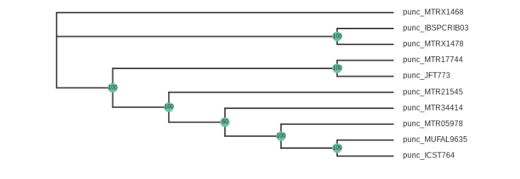
Rooting the tree
In the above figure the two Northern samples are nested deep within the Southern clade, but this tree is unrooted. Lets say we want to root the tree on the Northern samples and replot. This is accomplished by adding the root parameter to the tree.draw() function and specifying the samples to root the tree to:
tre = toytree.tree(rax.trees.bipartitions)
tre.draw(
    tre.root(["punc_ICST764", "punc_MUFAL9635"]),
    width=600,
    node_labels=tre.get_node_values("support"),
);
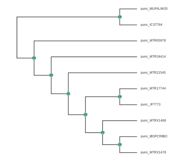
Note: The
root()function accepts a list of samples, so if you have multiple samples from the root taxon, you can include them like this:tre.root(["punc_ICST764", "punc_MUFAL9635", "punc_MTR05978"])
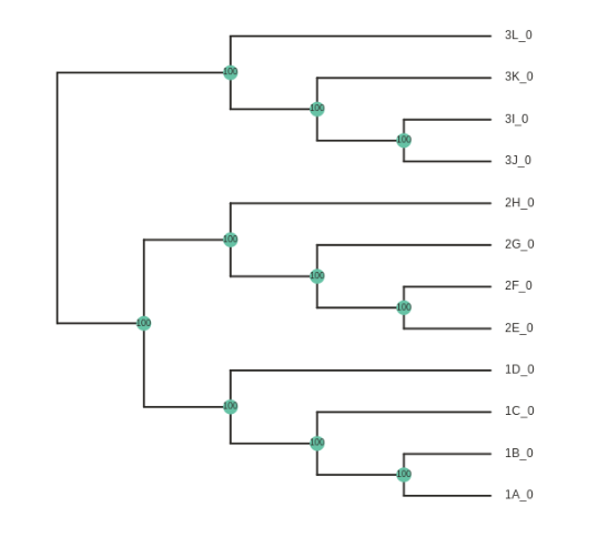
Experimenting with the simulated data
Tree rooting can also be accomplished with the wildcard parameter of the tree.root() function. This is somewhat more straightforward to demonstrate with the simulated data, so we can create a new raxml object with the simulated phylip file, rerun the RAxML tree inference, and then do some plotting:
rax = ipa.raxml(
    data="/scratch/af-biota/simrad-example/simrad_outfiles/simrad.phy",
    name="aligntest",
    workdir="./analysis-raxml",
    );

rax.params.N = 10
rax.params.T = 2
rax.params.o = None

rax.run(force=True)
Here the wildcard="3" argument specifies to root the tree using all the samples that include “3” in their names.
tre = toytree.tree(rax.trees.bipartitions)
tre.draw(
    tre.root(wildcard="3"),
    width=600,
    node_labels=tre.get_node_values("support"),
);
Further exploration
We provide a more thorough exploration of the ipyrad.analysis.raxml module in a notebook on the ipyrad github site, including more details about how to take full advantage of running parallel RAxML processes on a cluster.