Cluster Basics and Housekeeping
The bulk of the activities this morning involve getting oriented on the cluster and getting programs and resources set up for the actual assembly and analysis. We make no assumptions about prior experience with cluster environments, so we scaffold the entire participant workshop experience from first principles. More advanced users hopefully will find value in some of the finer details we present.
- Connecting to the cluster: Windows/Mac/Linux
- Basic command line navigation
- Setting up the computing environment
- Fetching the data
- Basic quality control (FastQC)
- Viewing and interpreting FAstQC results
Tutorial documentation conventions
Each grey cell in this tutorial indicates a command line interaction. Lines starting with $ indicate a command that should be executed in a terminal, for example by copying and pasting the text into your terminal. All lines in code cells beginning with ## are comments and should not be copied and executed. Elements in code cells surrounded by angle brackets (e.g. <username>) are variables that need to be replaced by the user. All other lines should be interpreted as output from the issued commands.
## Example Code Cell.
## Create an empty file in my home directory called `watdo.txt`
$ touch ~/watdo.txt

## Print "wat" to the screen
$ echo "wat"
wat
Columbia Habanero cluster information
Computational resources for the duration of this workshop have been generously provided by the Columbia University HPC facility, with special thanks to George Garrett for technical support. The cluster we will be using is located at habanero.rcs.columbia.edu. We have a reserved partition of the cluster for use in this workshop composed of five 24-core nodes. We will walk through instrutions for executing short or long running jobs on a cluster.
RADCamp NYC 2018 Participant Username/Port# List
SSH and the command line
Unlike laptop or desktop computers, cluster systems typically (almost exclusively) do not have graphical user input interfaces. Interacting with an HPC system therefore requires use of the command line to establish a connection, and for running programs and submitting jobs remotely on the cluster. To interact with the cluster through a terminal we use a program called SSH (secure shell) to create a fast and secure connection.
SSH for windows
Windows computers need to use a 3rd party app for connecting to remote computers. The best app for this in my experience is puTTY, a free SSH client. Right click and “Save link as” on the 64-bit binary executable link if you are using a PC.
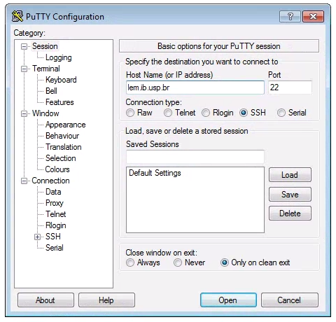
After installing puTTY, open it and you will see a box where you can enter the “Host Name (or IP Address)” of the computer you want to connect to (the ‘host’). To connect to the Habanero cluster, enter: habanero.rcs.columbia.edu. The default “Connection Type” should be “SSH”, and the default “Port” should be “22”. It’s good to verify these values. Leave everything else as defualt and click “Open”.
SSH for mac/linux
Linux operating systems come preinstalled with an ssh command line client, which we will assume linux users are aware of how to use. Mac computers are built on top of a linux-like operating system so they too ship with an SSH client, which can be accessed through the Terminal app. In a Finder window open Applications->Utilities->Terminal, then you can start an ssh session like this:
# enter your username here
$ ssh <username>@habanero.rcs.columbia.edu

# this is an example for the username "work2"
$ ssh work2@habanero.rcs.columbia.edu
Note on usage: In command line commands we’ll use the convention of wrapping variable names in angle-brackets. For example, in the command above you should substitute your own username for
<username>. We will provide usernames and passwords on the day of the workshop.
Command line interface (CLI) basics
The CLI provides a way to navigate a file system, move files around, and run commands all inside a little black window. The down side of CLI is that you have to learn many at first seemingly esoteric commands for doing all the things you would normally do with a mouse. However, there are several advantages of CLI: 1) you can use it on servers that don’t have a GUI interface (such as HPC clusters); 2) it’s scriptable, so you can write programs to execute common tasks or run analyses and others can easily reproduce these tasks exactly; 3) it’s often faster and more efficient than click-and-drag GUI interfaces. For now we will start with 4 of the most common and useful commands:
$ pwd
/home/work1
pwd stands for “print working directory”, which literally means “where am I now in this filesystem?”. This is a question you should always be aware of when working in a terminal. Just like when you open a file browser window, when you open a new terminal you are located somewhere; the terminal will usually start you out in your “home” directory. Ok, now we know where we are, lets take a look at what’s in this directory:
$ ls
ls stands for “list” and in our home directory there is not much, it appears! In fact right now there is nothing. This is okay, because you just got a brand new account, so you won’t expect to have anything there. Throughout the workshop we will be adding files and directories and by the time we’re done, not only will you have a bunch of experience with RAD-Seq analysis, but you’ll also have a ton of stuff in your home directory. We can start out by adding the first directory for this workshop:
$ mkdir ipyrad-workshop
mkdir stands for “make directory”, and unlike the other two commands, this command takes one “argument”. This argument is the name of the directory you wish to create, so here we direct mkdir to create a new directory called “ipyrad-workshop”. Now you can use ls again, to look at the contents of your home directory and you should see this new directory now:
$ ls
ipyrad-workshop
Throughout the workshop we will be introducing new commands as the need for them arises. We will pay special attention to highlighting and explaining new commands and giving examples to practice with.
Special Note: Notice that the above directory we are making is not called
ipyrad workshop. This is very important, as spaces in directory names are known to cause havoc on HPC systems. All linux based operating systems do not recognize file or directory names that include spaces because spaces act as default delimiters between arguments to commands. There are ways around this (for example Mac OS has half-baked “spaces in file names” support) but it will be so much for the better to get in the habit now of never including spaces in file or directory names.
Download and Install Software
Install conda
Conda is a command line software installation tool based on python. It will allow us to install and run various useful applications inside our home directory that we would otherwise have to hassle the HPC admins to install for us. Conda provides an isolated environment for each user, allowing us all to manage our own independent suites of applications, based on our own computing needs.
64-Bit Python2.7 conda installer for linux is here: https://repo.continuum.io/miniconda/Miniconda2-latest-Linux-x86_64.sh, so copy and paste this link into the commands as below:
$ wget https://repo.continuum.io/miniconda/Miniconda2-latest-Linux-x86_64.sh
Note:
wgetis a command line utility for fetching content from the internet. You use it when you want to get stuff from the web, so that’s why it’s calledwget.
After the download finishes you can execute the conda installer using bash. bash is the name of the terminal program that runs on the cluster, and .sh files are scripts that bash knows how to run. The extra argument -b at the end is specific to this .sh script, and tells it to automatically run the entire script (in batch mode) instead of stopping to ask us questions as it goes.
$ bash Miniconda2-latest-Linux-x86_64.sh -b
This will create a new directory where the conda program will be located, and also where all of the software that we will eventually install with conda will be stored. By default the new directory will be placed in your home directory and will be called miniconda2. After the install completes we will add this new directory to our PATH variable, which is what the terminal uses to recognize where software is located on your system. After running the commands below our terminal will always be able to find our conda software.
$ echo PATH='$HOME'/miniconda2/bin:'$PATH' >> ~/.bashrc
$ source ~/.bashrc
$ which python
/home/work1/miniconda2/bin/python
The echo command prints the text that comes after to it and the “»” character designates to write the result to the file .bashrc. This is a file that is automatically run when the terminal starts. If we had not run the miniconda installer in batch mode it would have appended this command to the .bashrc file for us automatically, but it takes longer that way so we are doing it by hand instead. The source command simply tells the terminal to reload the .bashrc file so that it is like we started a new terminal, but this time it will find all of our new conda software. Finally, the which command will show you the path (location) of the program printed after it. In this case we ask which python binary it finds, and you can see that it returns that the new version of python in our personal miniconda directory.
Install ipyrad and fastqc
Conda gives us access to an amazing array of analysis tools for both analyzing and manipulating all kinds of data. Here we’ll just scratch the surface by installing ipyrad, the RAD-Seq assembly and analysis tool that we’ll use throughout the workshop, and FastQC, an application for filtering fasta files based on several quality control metrics. As long as we’re installing conda packages we’ll include toytree as well, which is a plotting library used by the ipyrad analysis toolkit.
We’ll explain this part in more detail further below, but for now run the command below to connect to an interactive session on a compute node. This way we will not be using the head node of the cluster (shared resource) when we are all installing software simultaneously.
$ srun --pty -t 1:00:00 --account=edu --reservation=edu_23 /bin/bash
Now that you are connected to a compute node run the commands below:
$ conda install -c ipyrad ipyrad -y
$ conda install -c bioconda fastqc -y
$ conda install -c eaton-lab toytree -y
Note: The
-cflag indicates that we’re asking conda to fetch apps from theipyrad,bioconda, andeaton-labchannels. Channels are seperate repositories of apps maintained by independent developers.
After you type y to proceed with install, these commands will produce a lot of output that looks like this:
libxml2-2.9.8        |  2.0 MB | ################################################################################################################################# | 100%
expat-2.2.5          |  186 KB | ################################################################################################################################# | 100%
singledispatch-3.4.0 |   15 KB | ################################################################################################################################# | 100%
pandocfilters-1.4.2  |   12 KB | ################################################################################################################################# | 100%
pandoc-2.2.1         | 21.0 MB | ################################################################################################################################# | 100%
mistune-0.8.3        |  266 KB | ################################################################################################################################# | 100%
send2trash-1.5.0     |   16 KB | ################################################################################################################################# | 100%
gstreamer-1.14.0     |  3.8 MB | ################################################################################################################################# | 100%
qt-5.9.6             | 86.7 MB | ################################################################################################################################# | 100%
freetype-2.9.1       |  821 KB | ################################################################################################################################# | 100%
wcwidth-0.1.7        |   25 KB | ################################################################################################################################# | 100%
These (and many more) are all the dependencies of ipyrad and fastqc. Dependencies can include libraries, frameworks, and/or other applications that we make use of in the architecture of our software. Conda knows all about which dependencies will be needed and installs them automatically for you. Once the process is complete (may take several minutes), you can verify the install by asking what version of each of these apps is now available for you on the cluster.
$ ipyrad --version
ipyrad 0.7.28

$ fastqc --version
FastQC v0.11.7
Examine the raw data
Here we will get hands-on with real data for the first time. We provide three empirical data sets to choose from, and throughout the workshop we will often compare our results among the three. Each example data set is composed of a dozen or more closely related species or population samples. They are ordered in order of the average divergence among samples. The Anolis data set is a “population-level” data set; the Pedicularis data set is composed of several closely related species and subspecies; and the Finch data set includes several species of finches from two relatively distant clades.
- Prates et al. 2016 (Anolis, single-end GBS).
- Eaton et al. 2013 (Pedicularis, single-end RAD).
- DaCosta and Sorenson 2016 (Finches, single-end ddRAD).
- Simulated datasets
The raw data are located in a special shared folder on the HPC system where we can all access them. Any analyses we run will only read from these files (i.e., they are read-only), not modify them. This is typical of any bioinformatic analysis. We want to develop a set of scripts that start from the unprocessed data and end in new results or statistics. You can use ls to examine the data sets in the shared directory space.
$ ls /rigel/edu/radcamp/files/SRP021469
29154_superba_SRR1754715.fastq.gz       35855_rex_SRR1754726.fastq.gz
30556_thamno_SRR1754720.fastq.gz        38362_rex_SRR1754725.fastq.gz
30686_cyathophylla_SRR1754730.fastq.gz  39618_rex_SRR1754723.fastq.gz
32082_przewalskii_SRR1754729.fastq.gz   40578_rex_SRR1754724.fastq.gz
33413_thamno_SRR1754728.fastq.gz        41478_cyathophylloides_SRR1754722.fastq.gz
33588_przewalskii_SRR1754727.fastq.gz   41954_cyathophylloides_SRR1754721.fastq.gz
35236_rex_SRR1754731.fastq.gz
Inspect the data
Then we will use the zcat command to read lines of data from one of the files and we will trim this to print only the first 20 lines by piping the output to the head command. Using a pipe like this passes the output from one command to another and is a common trick in the command line.
Here we have our first look at a fastq formatted file. Each sequenced read is spread over four lines, one of which contains sequence and another the quality scores stored as ASCII characters. The other two lines are used as headers to store information about the read.
$ zcat /rigel/edu/radcamp/files/SRP021469/29154_superba_SRR1754715.fastq.gz | head -n 20
@29154_superba_SRR1754715.1 GRC13_0027_FC:4:1:12560:1179 length=74
TGCAGGAAGGAGATTTTCGNACGTAGTGNNNNNNNNNNNNNNGCCNTGGATNNANNNGTGTGCGTGAAGAANAN
+29154_superba_SRR1754715.1 GRC13_0027_FC:4:1:12560:1179 length=74
IIIIIIIGIIIIIIFFFFF#EEFE<?################################################
@29154_superba_SRR1754715.2 GRC13_0027_FC:4:1:15976:1183 length=74
TGCAGTTGTAAATACAAATATCCCAAAANNNNGNNNNNNNTNTAATATTTTGNAANNTTGAGGGGTGTGATNTN
+29154_superba_SRR1754715.2 GRC13_0027_FC:4:1:15976:1183 length=74
GGGGHHHHHHHHHHHHHDHGHHHHCAAA##############################################
@29154_superba_SRR1754715.3 GRC13_0027_FC:4:1:19092:1179 length=74
TGCAGGCTCTGACAAAGAANTCGACTGANNNNNNNNNNNNNNCACNGGTTCNNGNNNATGTCAATGTGGTANAN
+29154_superba_SRR1754715.3 GRC13_0027_FC:4:1:19092:1179 length=74
GGGGHHHHBHHBHEB?B@########################################################
@29154_superba_SRR1754715.4 GRC13_0027_FC:4:1:1248:1210 length=74
TGCAGAACTGCTCCCAGAATCTCCAGAAATTGCGAGATTACCCCCAAAATCTCCAGAAATTTCTAGATTACCTC
+29154_superba_SRR1754715.4 GRC13_0027_FC:4:1:1248:1210 length=74
HHHHHDHHHFHHHDHBGHGHHHHHHHGDHE<GGE<D>DGHGGHHHDHHHHHHGHHHHFHHHHHHEHGHHEDEF>
@29154_superba_SRR1754715.5 GRC13_0027_FC:4:1:5242:1226 length=74
TGCAGCAGTCACCAGTCTGGCCCCTACCTCACAAAGTAGCTTGATGGCCGAACCACTCCCAAGGTGAATAGTGC
+29154_superba_SRR1754715.5 GRC13_0027_FC:4:1:5242:1226 length=74
HHHHHHHHHGGGGGHHHGHHHGHGGGGGBHHHBHEE>BGADDDDFHEHFDBGBDCFHBHBB8DD4???::?::?
@29154_superba_SRR1754715.6 GRC13_0027_FC:4:1:12660:1232 length=74
TGCAGGCCCAAAATCAACAATTATGCATAATACAACAAAGTTAATTAATTAATTATATTAAAAAAAGAAAAAGA
+29154_superba_SRR1754715.6 GRC13_0027_FC:4:1:12660:1232 length=74
HHHHHHHHHHHHHHHHHHHHHHHHHHHHGGHHHHFHHHHHHHHHHHHHHHHHHHHHHHHHHHHHHHHHHHHHHH
FastQC for quality control
The first step of any RAD-Seq assembly is to inspect your raw data to estimate overall quality. We began first with a visual inspection above, but of course we can only visually inspect a very tiny proportion of the total data. So instead we use automated approaches to check the quality of our data.
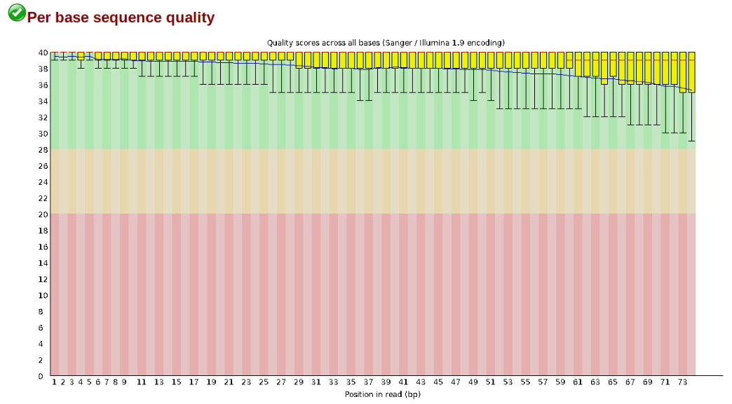
At this stage you can then attempt to improve your dataset by identifying and removing samples with failed sequencing. Another key QC procedure involves inspecting average quality scores per base position and trimming read edges, which is where low quality base-calls tend to accumulate. In this figure, the X-axis shows the position on the read in base-pairs and the Y-axis depicts information about Phred quality score per base for all reads, including median (center red line), IQR (yellow box), and 10%-90% (whiskers). As an example, here is a very clean base sequence quality report for a 75bp RAD-Seq library. These reads have generally high quality across their entire length, with only a slight (barely worth mentioning) dip toward the end of the reads:
In contrast, here is a somewhat typical base sequence quality report for R1 of a 300bp paired-end Illumina run of ezrad data:
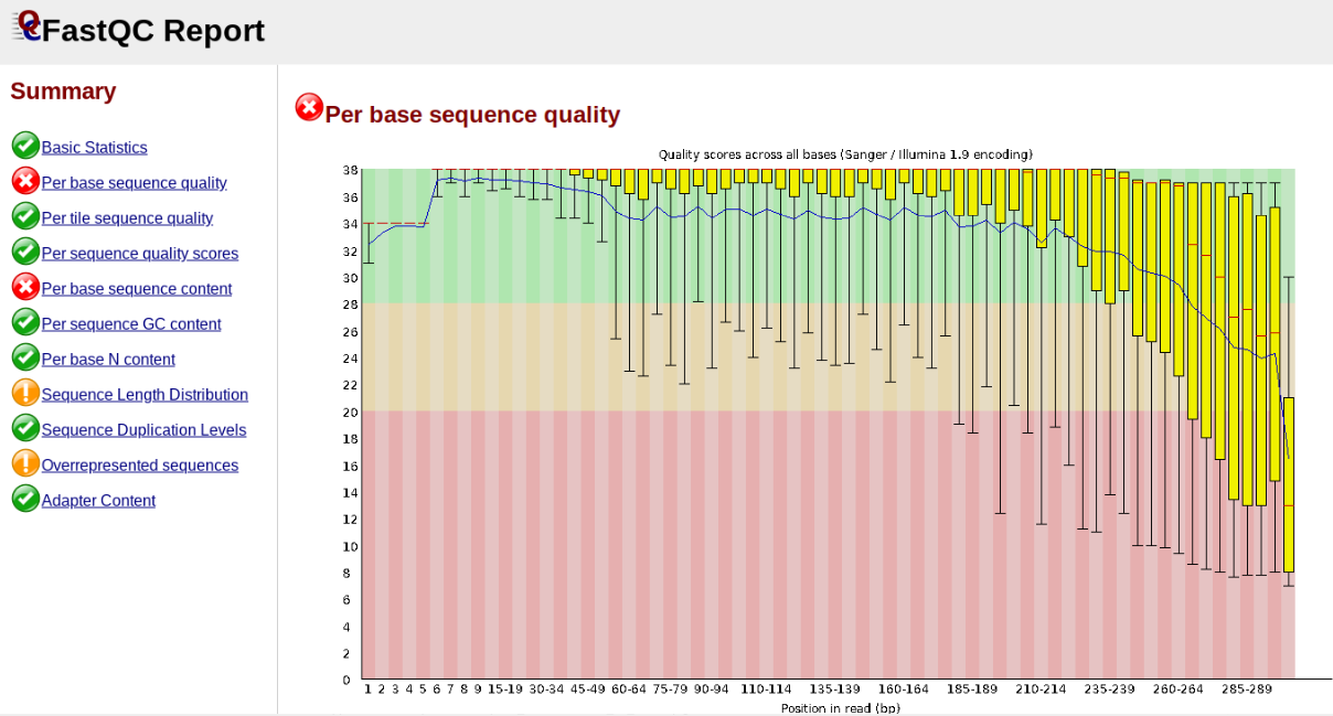
This figure depicts a common artifact of current Illumina chemistry, whereby quality scores per base drop off precipitously toward the ends of reads, with the effect being magnified for read lengths > 150bp. The purpose of using FastQC to examine reads is to determine whether and how much to trim our reads to reduce sequencing error interfering with basecalling. In the above figure, as in most real dataset, we can see there is a tradeoff between throwing out data to increase overall quality by trimming for shorter length, and retaining data to increase value obtained from sequencing with the result of increasing noise toward the ends of reads.
Running FastQC on the Anolis data
In preparation for running FastQC it is a good idea to keep yourself organized by creating an output directory to keep the FastQC results organized:
$ cd ~/ipyrad-workshop
$ mkdir fastqc-results
Now run fastqc on one of the samples:
$ fastqc -o fastqc-results /rigel/edu/radcamp/files/punc_IBSPCRIB0361_R1_.fastq.gz
Note: The
-oflag tells fastqc where to write output files. Especially Notice the relative path to the raw file. The difference between relative and absolute paths is an important one to learn. Relative paths are specified with respect to the current working directory. Since I am in/rigel/edu/radcamp/users/work1/ipyrad-workshop, and this is the directory therawsdirectory is in, I can simply reference it directly. If I was in any other directory I could specify the absolute path to the target fastq.gz file which would be/rigel/edu/radcamp/users/work1/ipyrad-workshop/raws/punc_IBSPCRIB0361_R1_.fastq.gz. Absolute paths are always more precise, but also always (often much) longer.
FastQC will indicate its progress in the terminal. This toy data will run quite quickly, but real data can take somewhat longer to analyse (10s of minutes).
Started analysis of punc_IBSPCRIB0361_R1_.fastq.gz
Approx 5% complete for punc_IBSPCRIB0361_R1_.fastq.gz
Approx 10% complete for punc_IBSPCRIB0361_R1_.fastq.gz
Approx 15% complete for punc_IBSPCRIB0361_R1_.fastq.gz
Approx 20% complete for punc_IBSPCRIB0361_R1_.fastq.gz
Approx 25% complete for punc_IBSPCRIB0361_R1_.fastq.gz
Approx 30% complete for punc_IBSPCRIB0361_R1_.fastq.gz
Approx 35% complete for punc_IBSPCRIB0361_R1_.fastq.gz
Approx 40% complete for punc_IBSPCRIB0361_R1_.fastq.gz
Approx 45% complete for punc_IBSPCRIB0361_R1_.fastq.gz
Approx 50% complete for punc_IBSPCRIB0361_R1_.fastq.gz
Approx 55% complete for punc_IBSPCRIB0361_R1_.fastq.gz
Approx 60% complete for punc_IBSPCRIB0361_R1_.fastq.gz
Approx 65% complete for punc_IBSPCRIB0361_R1_.fastq.gz
Approx 70% complete for punc_IBSPCRIB0361_R1_.fastq.gz
Approx 75% complete for punc_IBSPCRIB0361_R1_.fastq.gz
Approx 80% complete for punc_IBSPCRIB0361_R1_.fastq.gz
Approx 85% complete for punc_IBSPCRIB0361_R1_.fastq.gz
Approx 90% complete for punc_IBSPCRIB0361_R1_.fastq.gz
Approx 95% complete for punc_IBSPCRIB0361_R1_.fastq.gz
Approx 100% complete for punc_IBSPCRIB0361_R1_.fastq.gz
Analysis complete for punc_IBSPCRIB0361_R1_.fastq.gz
If you feel so inclined you can QC on all the raw data files in a folder by using a wildcard substitution:
$ fastqc -o fastqc-results /rigel/edu/radcamp/files/SRP021469/*.gz
Note: The
*here is a special command line character that means “Everything that matches this pattern”. So hereSRP021469/*matches everything in the raws directory. Equivalent (though more verbose) statements are:ls SRP021469/*.gz,ls SRP021469/*.fastq.gz. All of these will list all the files in theSRP021469directory. Special Challenge: Can you construct anlscommand using wildcards that only lists samples in theSRP021469directory that include the digit 5 in their sample name?
Examining the output directory you’ll see something like this (here we use ls -l to list the results in a more easily readable list form:
$ ls -l fastqc-results/
-rw-r--r-- 1 work1 habaedu 337122 Aug 28 08:21 29154_superba_SRR1754715_fastqc.html
-rw-r--r-- 1 work1 habaedu 494465 Aug 28 08:21 29154_superba_SRR1754715_fastqc.zip
-rw-r--r-- 1 work1 habaedu 336908 Aug 28 08:21 30556_thamno_SRR1754720_fastqc.html
-rw-r--r-- 1 work1 habaedu 494957 Aug 28 08:21 30556_thamno_SRR1754720_fastqc.zip
-rw-r--r-- 1 work1 habaedu 346060 Aug 28 08:22 30686_cyathophylla_SRR1754730_fastqc.html
-rw-r--r-- 1 work1 habaedu 508578 Aug 28 08:22 30686_cyathophylla_SRR1754730_fastqc.zip
-rw-r--r-- 1 work1 habaedu 345129 Aug 28 08:22 32082_przewalskii_SRR1754729_fastqc.html
-rw-r--r-- 1 work1 habaedu 506727 Aug 28 08:22 32082_przewalskii_SRR1754729_fastqc.zip
-rw-r--r-- 1 work1 habaedu 337555 Aug 28 08:22 33413_thamno_SRR1754728_fastqc.html
-rw-r--r-- 1 work1 habaedu 496787 Aug 28 08:22 33413_thamno_SRR1754728_fastqc.zip
-rw-r--r-- 1 work1 habaedu 336544 Aug 28 08:23 33588_przewalskii_SRR1754727_fastqc.html
-rw-r--r-- 1 work1 habaedu 494611 Aug 28 08:23 33588_przewalskii_SRR1754727_fastqc.zip
-rw-r--r-- 1 work1 habaedu 329055 Aug 28 08:23 35236_rex_SRR1754731_fastqc.html
-rw-r--r-- 1 work1 habaedu 483019 Aug 28 08:23 35236_rex_SRR1754731_fastqc.zip
-rw-r--r-- 1 work1 habaedu 333034 Aug 28 08:23 35855_rex_SRR1754726_fastqc.html
-rw-r--r-- 1 work1 habaedu 489218 Aug 28 08:23 35855_rex_SRR1754726_fastqc.zip
-rw-r--r-- 1 work1 habaedu 341427 Aug 28 08:23 38362_rex_SRR1754725_fastqc.html
-rw-r--r-- 1 work1 habaedu 500975 Aug 28 08:23 38362_rex_SRR1754725_fastqc.zip
-rw-r--r-- 1 work1 habaedu 334602 Aug 28 08:24 39618_rex_SRR1754723_fastqc.html
-rw-r--r-- 1 work1 habaedu 489714 Aug 28 08:24 39618_rex_SRR1754723_fastqc.zip
-rw-r--r-- 1 work1 habaedu 342964 Aug 28 08:24 40578_rex_SRR1754724_fastqc.html
-rw-r--r-- 1 work1 habaedu 503731 Aug 28 08:24 40578_rex_SRR1754724_fastqc.zip
-rw-r--r-- 1 work1 habaedu 342211 Aug 28 08:25 41478_cyathophylloides_SRR1754722_fastqc.html
-rw-r--r-- 1 work1 habaedu 503054 Aug 28 08:25 41478_cyathophylloides_SRR1754722_fastqc.zip
-rw-r--r-- 1 work1 habaedu 336088 Aug 28 08:26 41954_cyathophylloides_SRR1754721_fastqc.html
-rw-r--r-- 1 work1 habaedu 494066 Aug 28 08:26 41954_cyathophylloides_SRR1754721_fastqc.zip
Now we have output files that include html and images depicting lots of information about the quality of our reads, but we can’t inspect these because we only have a CLI interface on the cluster. How do we get access to the output of FastQC?
Obtaining FastQC Output (scp) (linux/MacOSX)
You can use the scp tool to copy files from the cluster to your local computer so that you can visualize the results on your graphical user interface on your computer. Take note of the . at the end of the command and the need to substitute your username (e.g., work3) into the command.
# run this from a terminal on your local computer (not connected to the cluster)
scp -r <username>@habanero.rcs.columbia.edu:/rigel/edu/radcamp/users/<username>/ipyrad-workshop/fastq-results .
Or, obtaining FastQC output (Windows)
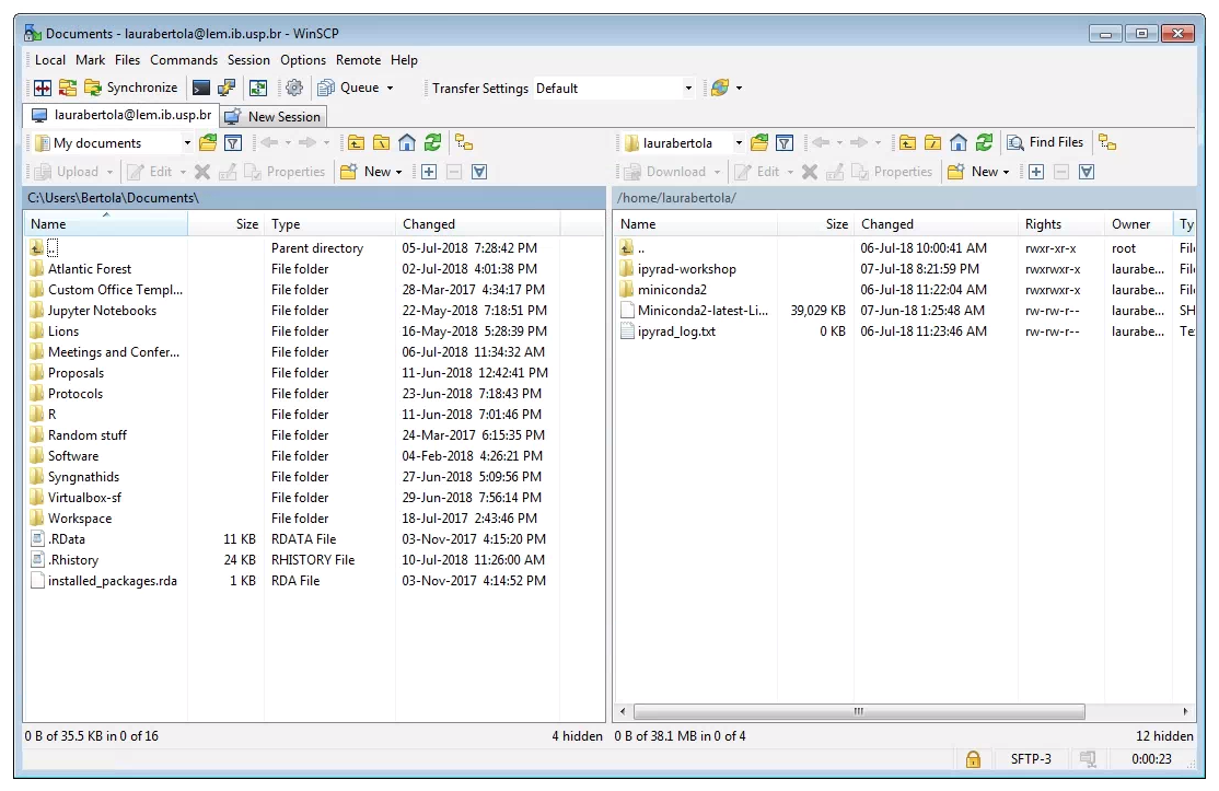
Moving files between the cluster and your local computer is a very common task, and this will typically be accomplished with a secure file transfer protocol (sftp) client. Various Free/Open Source GUI tools exist but we recommend WinSCP for Windows.
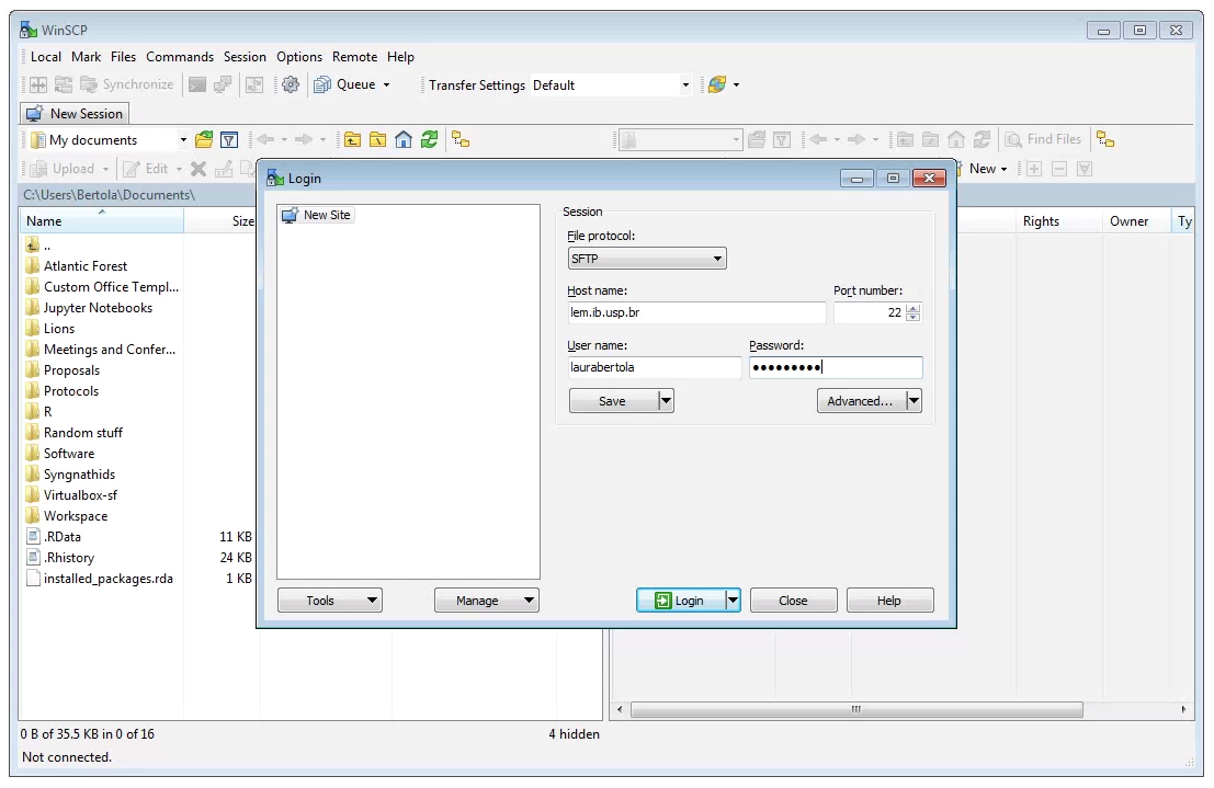
After downloading, installing, and opening WinSCP, you will see the following screen. First, ensure that the “File Protocol is set to “SFTP”. The connection will fail if “SFTP” is not chosen her. Next, fill out the host name (habanero.rcs.columbia.edu), your username and password, and click “Login”.
 Two windows file browsers will appear: your laptop on the left, and the cluster on the right. You can navigate through the folders and transfer files from the cluster to your laptop by dragging and dropping them.
Inspecting and Interpreting FastQC Output
Once the files are downloaded you can now open them on your local computer like normal by double clicking on the .html files which will open in a browser.
Just taking a random one, lets spend a moment looking at the results from punc_JFT773_R1__fastqc.html. Opening up this html file, on the left you’ll see a summary of all the results, which highlights areas FastQC indicates may be worth further examination. We will only look at a few of these.
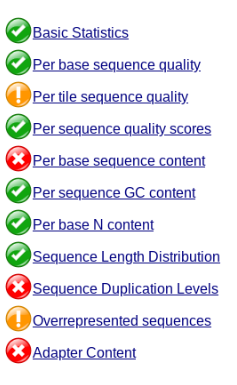
Lets start with Per base sequence quality, because it’s very easy to interpret, and often times with RAD-Seq data results here will be of special importance.
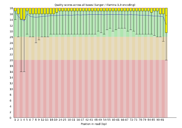
For the Anolis data the sequence quality per base is uniformly quite high, with dips only in the first and last 5 bases (again, this is typical for Illumina reads). Based on information from this plot we can see that the Anolis data doesn’t need a whole lot of trimming, which is good.
Now lets look at the Per base sequece content, which FastQC highlights with a scary red X.
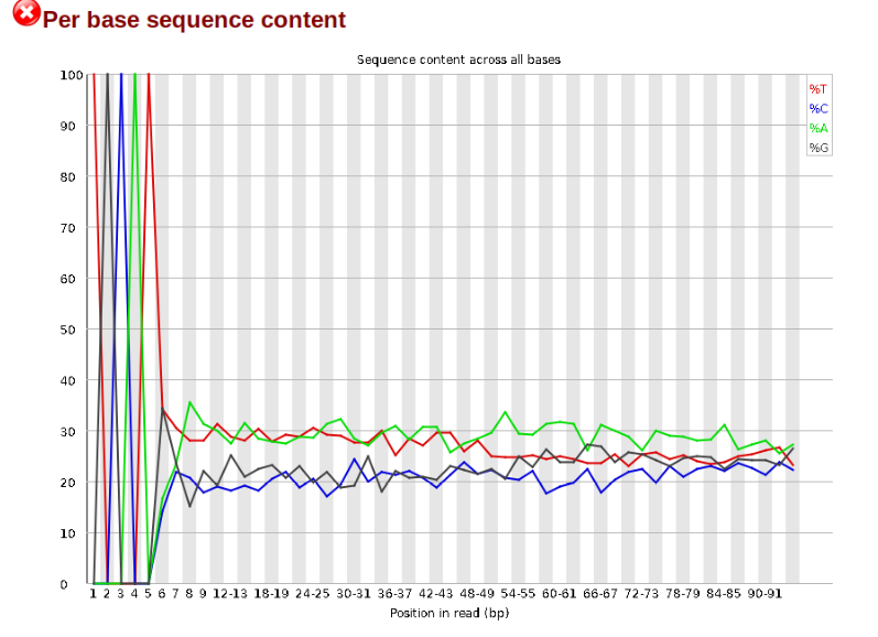
The squiggles indicate base composition per base position averaged across the reads. It looks like the signal FastQC is concerned about here is related to the extreme base composition bias of the first 5 positions. We happen to know this is a result of the restriction enzyme overhang present in all reads (TGCAT in this case for the EcoT22I enzyme used), and so it is in fact of no concern. Now lets look at Adapter Content:
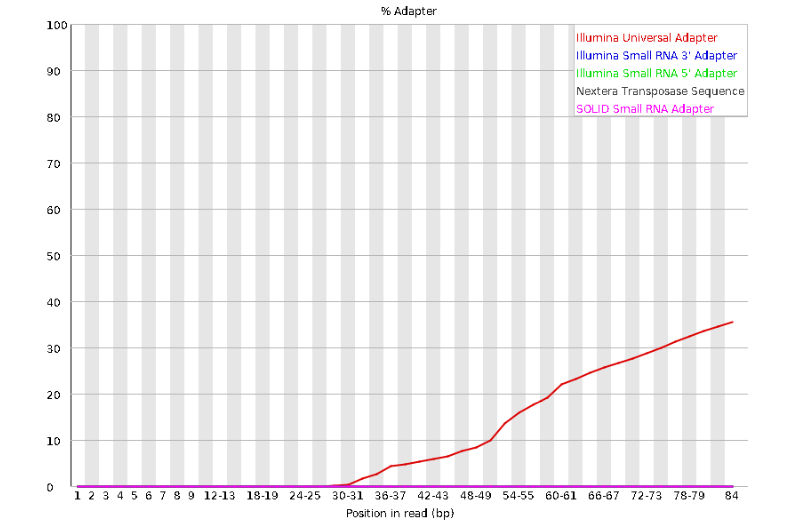
Here we can see adapter contamination increases toward the tail of the reads, approaching 40% of total read content at the very end. The concern here is that if adapters represent some significant fraction of the read pool, then they will be treated as “real” data, and potentially bias downstream analysis. In the Anolis data this looks like it might be a real concern so we shall keep this in mind during step 2 of the ipyrad analysis, and incorporate 3’ read trimming and aggressive adapter filtering.
Other than this, the data look good and we can proceed with the ipyrad analysis.
References
Elshire, R. J., Glaubitz, J. C., Sun, Q., Poland, J. A., Kawamoto, K., Buckler, E. S., & Mitchell, S. E. (2011). A robust, simple genotyping-by-sequencing (GBS) approach for high diversity species. PloS one, 6(5), e19379.
Prates, I., Xue, A. T., Brown, J. L., Alvarado-Serrano, D. F., Rodrigues, M. T., Hickerson, M. J., & Carnaval, A. C. (2016). Inferring responses to climate dynamics from historical demography in neotropical forest lizards. Proceedings of the National Academy of Sciences, 113(29), 7978-7985.