Demographic inference using the Site Frequency Spectrum (SFS) with momi2
What is the SFS?
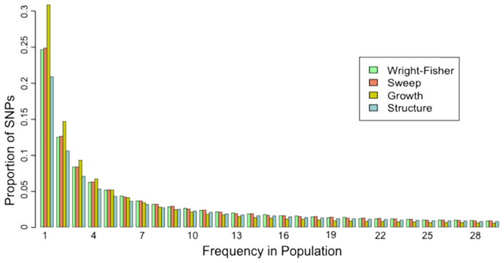
The site frequency spectrum (SFS) is a histogram of the frequencies of SNPs in a sample of individuals from a population. Different population histories leave characteristic signatures on the SFS. For example, a population that has undergone a recent bottleneck will have a reduced number of rare variants as compared to a neutrally evolving population. Rare variants will be lost much more rapidly than common variants under a bottleneck model. On the other hand, population expansion models will display an excess of rare variants with respect to a neutral model. In a similar fashion, selection and gene flow can leave characteristic imprints on the SFS of a population. A good example of how the SFS is calculated can be found on wikipedia.
What is demographic inference?
The goal of demographic analyses is to understand the history of lineages (sometimes referred as ‘populations’) in a given species, estimating the neutral population dynamics such as time of divergence, population expansion, population contraction, bottlenecks, admixture, etc. A nice example of a paper that performs model selection and parameter estimation is Portik et al 2017.
Most importantly, how do you pronounce momi?
Pronunciation: Care of Jonathan Terhorst (somewhat cryptically), from a github issue I created to resolve this conundrum: “How do you pronounce ∂a∂i? ;-)”…. And another perspective from Jack Kamm: “Both pronunciations are valid, but I personally say ‘mommy’”.
Setting up the momi environment (TL;DR)
(NB: All the -c arguments again are specifying channels that momi2 pulls
dependencies from. Order matters here, so copy and paste this command to your
terminal).
$ conda create -n momi_py36 python=3.6 -y
$ conda activate momi_py36
$ conda install momi ipyparallel openblas jupyter -c defaults -c conda-forge -c bioconda -c jackkamm -y
This will produce copious output, and should take <5 minutes.
momi2 Analyses
Create a new notebook called simdata-momi2.ipynb. The rest of the materials
in this part of the workshop assume you are running all code in cells of a
jupyter notebook.
- Constructing and plotting a simple model
- Preparing real data for analysis
- Inference procedure
- Bootstrapping confidence intervals
Constructing and plotting a simple model
One of the real strengths of momi2 is the ability not only to construct a demographic history for a set of populations, but also to plot the model to verify that it corresponds to what you expect!
Begin with the usual import statements, except this time we also add logging,
which allows momi2 to write progress to a log file. This can be useful for
debugging, so we encourage this practice.
%matplotlib inline
import momi		## momi2 analysis
import logging		## create log file

logging.basicConfig(level=logging.INFO,
                    filename="momi_log.txt")
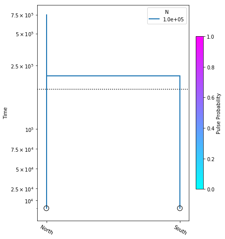
A demographic model is composed of leaf nodes, migration events,
and size change events. We start with the simplest possible 2
population model, with no migration, and no size changes. For the
sake of demonstrating model construction we choose arbitrary
values for N_e (the diploid effective size), and t (the time
at which all lineages move from the “South” population to the
“North” population).
model = momi.DemographicModel(N_e=1e5)
model.add_leaf("North")
model.add_leaf("South")
model.move_lineages("South", "North", t=2e5)
Note: The default migration fraction of the
DemographicModel.move_lineages()function is 100%, so if we do not specify this value then when we callmove_lineagesmomi2 assumes we want to move all lineages from the source to the destination. Later we will see how to manipulate the migration fraction to only move some portion of lineages.
Executing this cell produces no output, but that’s okay, we are just specifying the model. Also, be aware that the names assigned to leaf nodes have no specific meaning to momi2, so these names should be selected to have specific meaning to your target system. Here “North” and “South” are simply stand-ins for some hypothetical populations. Now that we have this simple demographic model parameterized we can plot it, to see how it looks.
yticks = [1e4, 2.5e4, 5e4, 7.5e4, 1e5, 2.5e5, 5e5, 7.5e5]

fig = momi.DemographyPlot(
    model,
    ["North", "South"],
    figsize=(6,8),
    major_yticks=yticks,
    linthreshy=1e5)
There’s a little bit going on here, but we’ll walk you through it:
yticks- This is a list of elements specifying the timepoints to highlight on the y-axis of the figure.
The first two arguments to momi.DemographyPlot() are required, namely the model
to plot, and the populations of the model to include. The next three arguments are
optional, but useful:
figsize- Specify the output figure size as (width, height) in inches.major_yticks- Tells the momi2 plotting routine to use the time demarcations we specified in thieyticksvariable.linthreshy- The time point at which to switch from linear to log-scale, backwards in time. This is really useful if you have many “interesting” events happening relatively recently, and you don’t want them to get “smooshed” together by the depth of the older events. This will become clearer as we add migration events later in the tutorial.
Experiment: Try changing the value of linthreshy and replotting. Try 1e4
and 1.5e5 and notice how the figure changes. You can also experiment with
changing the values in the yticks list.
Let’s create a new model and introduce one migration event that only moves some fraction of lineages, and not the totality of them:
model = momi.DemographicModel(N_e=1e5)

model.add_leaf("North")
model.add_leaf("South")
model.move_lineages("South", "North", p=0.1, t=5e4)
model.move_lineages("South", "North", t=2e5)

yticks = [1e4, 2.5e4, 5e4, 7.5e4, 1e5, 2.5e5, 5e5, 7.5e5]

fig = momi.DemographyPlot(
    model, ["North", "South"],
    figsize=(6,8),
    major_yticks=yticks,
    linthreshy=1.5e5)
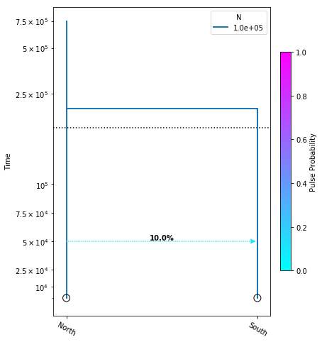
This is almost the exact same model as above, except now we have introduced
another move_lineages call which includes the p=0.1 argument. This
indicates that we wish to move 10% of lineages from the “South” population
to the “North” population at the specified timepoint.
Note: It may seem odd that the arrow in this figure points from “North” to “South”, but this is simply because we are operating in a coalescent framework and therefore the
move_lineagesfunction operates backwards in time.
Experiment: Try adding a third leaf node, and replotting. Call the new leaf “Central”.
Simulating data under your desired model.
Momi2 provides a really convenient function for generating data under a model, once you’re happy with the model you’ve specified.
## Specify how many haploid samples per population you want to simulate
sampled_n_dict={"North":4, "South":4}

model.simulate_vcf(out_prefix="momi_simdata",
                    length=1e5,
                    recoms_per_gen=1e-8,
                    muts_per_gen=1e-8,
                    chrom_name="chr1",
                    ploidy=2,
                    sampled_n_dict=sampled_n_dict)
Now in your radcamp-tmp directory you’ll see three new files:
!ls -1 ~/radcamp-tmp
momi_simdata.bed
momi_simdata.vcf.gz
momi_simdata.vcf.gz.tbi
Taking a quick peek at the vcf file you can verify the typical structure of a vcf file, and that we have 2 diploid samples each from North and South (you can also see that momi2 vcf is phased):
zcat momi_simdata.vcf.gz | head -n 24
##fileformat=VCFv4.2
##source="VCF simulated by momi2 using msprime backend"
##contig=<ID=chr1,length=100000.0>
##FORMAT=<ID=GT,Number=1,Type=String,Description="Genotype">
##INFO=<ID=AA,Number=1,Type=String,Description="Ancestral Allele">
#CHROM  POS     ID      REF     ALT     QUAL    FILTER  INFO    FORMAT  North_0 North_1 South_0 South_1
chr1    32      .       A       T       .       .       AA=A    GT      0|0     1|1     0|0     1|0
chr1    47      .       A       T       .       .       AA=A    GT      0|1     0|0     0|0     0|0
chr1    60      .       A       T       .       .       AA=A    GT      0|0     1|1     0|0     1|0
chr1    146     .       A       T       .       .       AA=A    GT      1|1     0|0     0|0     0|0
chr1    154     .       A       T       .       .       AA=A    GT      0|0     0|0     0|0     1|0
chr1    167     .       A       T       .       .       AA=A    GT      0|0     1|1     0|0     0|0
chr1    168     .       A       T       .       .       AA=A    GT      0|0     1|1     0|0     0|0
chr1    175     .       A       T       .       .       AA=A    GT      0|0     0|0     1|1     0|0
chr1    212     .       A       T       .       .       AA=A    GT      0|0     1|1     0|0     0|0
chr1    222     .       A       T       .       .       AA=A    GT      0|0     1|1     0|0     1|0
chr1    227     .       A       T       .       .       AA=A    GT      0|0     1|1     0|0     1|0
chr1    233     .       A       T       .       .       AA=A    GT      0|0     0|0     1|0     0|0
chr1    243     .       A       T       .       .       AA=A    GT      0|0     0|0     1|1     0|1
chr1    309     .       A       T       .       .       AA=A    GT      1|1     1|1     0|0     1|1
chr1    322     .       A       T       .       .       AA=A    GT      0|0     0|0     1|1     0|0
chr1    393     .       A       T       .       .       AA=A    GT      0|1     0|0     0|0     0|1
chr1    419     .       A       T       .       .       AA=A    GT      1|0     1|1     1|1     1|0
chr1    439     .       A       T       .       .       AA=A    GT      0|1     0|0     0|0     0|0
Preparing real data for analysis
In order to simplify this tutorial analysis we’ll use a subset of the Prates et al. 2016 dataset (which will enable a nice 2 population model). First, we need to gather and construct several input files before we can actually apply momi2 to our Anolis data.
- Population assignment file - This is a tab or space separated list of sample names and population names to which they are assigned. Sample names need to be exactly the same as they are in the VCF file. Population names can be anything, but it’s useful if they’re meaningful.
- Properly formatted VCF - We do have the VCF file output from the ipyrad Anolis assembly, but it requires a bit of massaging before it’s ready for momi2. It must be zipped and indexed in such a way as to make it searchable.
- BED file - This file specifies genomic regions to include in when calculating the SFS. It is composed of 3 columns which specify ‘chrom’, ‘chromStart’, and ‘chromEnd’.
- The allele counts file - The allele counts file is an intermediate file that we must generate on the way to constructing the SFS. momi2 provides a function for this.
- Genereate the SFS - The culmination of all this housekeeping is the SFS file which we will use for demographic inference.
Population assignment file
Based on the results of a PCA and also our knowledge of the geographic location
of the samples we will assign 2 samples to the “North” population, and 8 samples
to the “South” population. To save some time we created this pops file, and have
stashed a copy in the IBS RADCamp site. We can simply copy the file
from there into our own work directories.
%%bash
wget https://radcamp.github.io/Yale2019/Prates_et_al_2016_example_data/anolis_pops.txt
cat anolis_pops.txt
punc_ICST764    North
punc_MUFAL9635  North
punc_IBSPCRIB0361       South
punc_JFT773     South
punc_MTR05978   South
punc_MTR17744   South
punc_MTR21545   South
punc_MTR34414   South
punc_MTRX1468   South
punc_MTRX1478   South
Note: the
%%bashheader inside a notebook cell is amagiccommand that indicates to interpret everything in that shell as linux commands rather than python.
Properly formatted VCF
In this tutorial we are using a very small dataset, so manipulating the VCF is very
fast. With real data the VCF file can be enormous, which makes processing it
very slow. momi2 expects very large input files, so it insists on having them
preprocessed to speed things up. The details of this preprocessing step are not
very interesting, but we are basically compressing and indexing the VCF so it’s
faster to search.
%%bash
## fetch the vcf from the radcamp site
wget https://radcamp.github.io/Yale2019/Prates_et_al_2016_example_data/anolis.vcf

## bgzip performs a blockwise compression
## The -c flag directs bgzip to leave the original vcf file
##   untouched and create a new file for the vcf.gz
bgzip -c anolis.vcf > anolis.vcf.gz

## tabix indexes the file for searching
tabix anolis.vcf.gz
ls anolis/*
anolis_pops.txt anolis.vcf anolis.vcf.gz anolis.vcf.gz.tbi
BED file
The last file we need to construct is a BED file specifying which genomic regions to retain for calculation of the SFS. The standard coalescent assumes no recombination and no natural selection, so drift and mutation are the only forces impacting allele frequencies in populations. If we had whole genome data, and a good reference sequence then we would have information about coding regions and other things that are probably under selection, so we could use the BED file to exclude these regions from the analysis. With RAD-Seq type data it’s very common to assume RAD loci are neutrally evolving and unlinked, so we just want to create a BED file that specifies to retain all our SNPs. We provide a simple python program to do this conversion, which is located on github:
%%bash
wget https://raw.githubusercontent.com/isaacovercast/lab-notebooks/master/vcf2bed/vcf2bed.py

python vcf2bed.py anolis.vcf

## Print the first 10 lines of this file
head anolis.bed
locus_6 2       3
locus_6 40      41
locus_6 67      68
locus_6 68      69
locus_6 69      70
locus_6 70      71
locus_7 8       9
locus_7 33      34
locus_7 48      49
locus_7 51      52
The allele counts object
The allele counts object is an intermediate step necessary for generating the SFS.
It’s a format internal to momi2, so we won’t spend a lot of time describing it,
except to say that it is exactly what it says it is: A count of alleles in each
population. Since each diploid individual has 2 alleles per snp, the total count
of alleles per population will be 2n at maximum, and 0 at minimum.
## The population assignments transformed into a sample-to-population dictionary
ind2pop = {'punc_IBSPCRIB0361': 'South', 'punc_MTR05978': 'South', 'punc_MTR21545': 'South', 'punc_JFT773': 'South', 'punc_MTR17744': 'South', 'punc_MTR34414': 'South', 'punc_MTRX1478': 'South', 'punc_MTRX1468': 'South', 'punc_ICST764': 'North', 'punc_MUFAL9635': 'North'}

## Create the snp allele counts array
anolis_ac = momi.SnpAlleleCounts.read_vcf("anolis.vcf.gz", ancestral_alleles=False, bed_file="anolis.bed", ind2pop=ind2pop)
Generate the SFS
The momi site frequency spectrum is represented somewhat differently than you
might be used to if you have used dadi or fastsimcoal2. Here we load the SFS
generated above into the sfs object and print a few properties.
sfs = anolis_ac.extract_sfs(n_blocks=50)
print(sfs.n_snps())
print("Avg pairwise heterozygosity", sfs.avg_pairwise_hets[:5])
print("populations", sfs.populations)
print("percent missing data per population", sfs.p_missing)
Inference procedure
In the previous examples where we constructed and plotted DemographicModels, we had specified all the values for population sizes, divergence times, and migration fractions. This is useful when we are developing the models we want to test, because we can construct the model with toy parameter values, plot it and then visually inspect whether the model meets our expectations. Once we have settled on one or a handful of models to test, we can incorporate the observed SFS in an inference procedure in order to test which model is the best fit to the data. The best fitting model will then provide a set of maximum likelihood parameter values for the parameters we are interested in (like divergence time). We can then perform a bootstrap analysis, by randomly resampling the observed SFS, re-estimating parameters under the most likely model, and constructing bootstrap confidence intervals on these values (typically 50-100 replicates, but here 10 for speed).
Here we will invesigate three different 2 population models:
no_migration_model- All parameters fixed, except divergence time.pop_sizes_model- North and South populations are allowed to have different, variable sizes. Here we also estimate divergence time.migration_model- Allow one pulse of migration in both directions, at possibly different times, and with different migration fractions. Also, include all other parameters above (population sizes and divergence time).
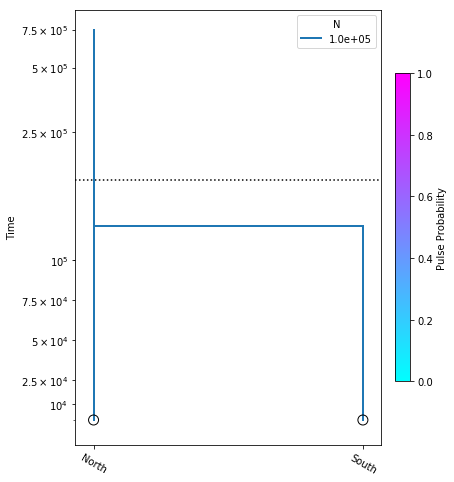
Estimating divergence time
Here we construct the no_migration_model, where we are estimating only
divergence time. We perform the optimization, and plot the model with the
resulting most likely parameter value.
no_migration_model = momi.DemographicModel(N_e=1e5)

no_migration_model.set_data(sfs)

no_migration_model.add_time_param("tdiv")

no_migration_model.add_leaf("North")
no_migration_model.add_leaf("South")
no_migration_model.move_lineages("South", "North", t="tdiv")

no_migration_model.optimize()
            fun: 0.6331043898321572
            jac: array([-2.03580439e-13])
  kl_divergence: 0.6331043898321572
 log_likelihood: -252.5589124720131
        message: 'Converged (|f_n-f_(n-1)| ~= 0)'
           nfev: 11
            nit: 3
     parameters: ParamsDict({'tdiv': 121612.07225824424})
         status: 1
        success: True
              x: array([121612.07225824])
yticks = [1e4, 2.5e4, 5e4, 7.5e4, 1e5, 2.5e5, 5e5, 7.5e5]

fig = momi.DemographyPlot(
    no_migration_model, ["North", "South"],
    figsize=(6,8),
    major_yticks=yticks,
    linthreshy=1.5e5)
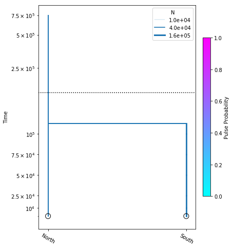
Including population size parameters
Here we construct the popsizes_model, where we are estimating variable
population sizes as well as divergence time. We perform the optimization,
and plot the model with the resulting most likely parameter values.
popsizes_model = momi.DemographicModel(N_e=1e5)

popsizes_model.set_data(sfs)

popsizes_model.add_size_param("n_north")
popsizes_model.add_size_param("n_south")
popsizes_model.add_time_param("tdiv")

popsizes_model.add_leaf("North", N="n_north")
popsizes_model.add_leaf("South", N="n_south")
popsizes_model.move_lineages("South", "North", t="tdiv")

popsizes_model.optimize()
           fun: 0.6080302639574219
           jac: array([-7.11116810e-06,  1.25870299e-06,  5.18524040e-11])
 kl_divergence: 0.6080302639574219
log_likelihood: -248.84794184255227
       message: 'Converged (|f_n-f_(n-1)| ~= 0)'
          nfev: 13
           nit: 6
    parameters: ParamsDict({'n_north': 58437.32067443618, 'n_south': 132874.21082953943, 'tdiv': 112867.76818828644})
        status: 1
       success: True
             x: array([1.09757100e+01, 1.17971582e+01, 1.12867768e+05])
yticks = [1e4, 2.5e4, 5e4, 7.5e4, 1e5, 2.5e5, 5e5, 7.5e5]

fig = momi.DemographyPlot(
    popsizes_model, ["North", "South"],
    figsize=(6,8),
    major_yticks=yticks,
    linthreshy=1.5e5)
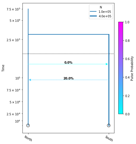
Adding migration events
migration_model = momi.DemographicModel(N_e=1e5)

migration_model.set_data(sfs)

migration_model.add_time_param("tmig_north_south")
migration_model.add_time_param("tmig_south_north")
migration_model.add_pulse_param("mfrac_north_south", upper=.2)
migration_model.add_pulse_param("mfrac_south_north", upper=.2)

migration_model.add_size_param("n_north")
migration_model.add_size_param("n_south")
migration_model.add_time_param("tdiv", lower_constraints=["tmig_north_south", "tmig_south_north"])

migration_model.add_leaf("North", N="n_north")
migration_model.add_leaf("South", N="n_south")
migration_model.move_lineages("North", "South", t="tmig_north_south", p="mfrac_north_south")
migration_model.move_lineages("South", "North", t="tmig_south_north", p="mfrac_south_north")


migration_model.move_lineages("South", "North", t="tdiv")

migration_model.optimize()
            fun: 0.6072433390803555
            jac: array([-4.44751606e-11,  1.40562352e-11, -2.46501280e-04,  1.24640859e-08,
       -2.14858289e-08,  2.17343690e-12,  1.43063167e-11])
  kl_divergence: 0.6072433390803555
 log_likelihood: -248.73147696074645
        message: 'Converged (|f_n-f_(n-1)| ~= 0)'
           nfev: 31
            nit: 8
     parameters: ParamsDict({'tmig_north_south': 95596.04975739817, 'tmig_south_north': 128584.2961865477, 'mfrac_north_south': 0.2, 'mfrac_south_north': 5.497639676362986e-07, 'n_north': 101409.03648320214, 'n_south': 274995.4822711156, 'tdiv': 300936.29078211787})
         status: 1
        success: True
              x: array([ 9.55960498e+04,  1.28584296e+05, -1.38629436e+00, -1.44137763e+01,
        1.15269175e+01,  1.25245099e+01,  1.72351995e+05])
yticks = [1e4, 2.5e4, 5e4, 7.5e4, 1e5, 2.5e5, 5e5, 7.5e5]

fig = momi.DemographyPlot(
    migration_model, ["North", "South"],
    figsize=(6,8),
    major_yticks=yticks,
    linthreshy=1.5e5)
Model selection with AIC
Model selection is typically performed with AIC, so here we extract the log likelihood of each model, calculate the AIC, and then calculate delta AIC values, and AIC weights. The best model will have the lowest AIC score. Delta AIC, and the AIC weight are indications of how confident we can be that the best fitting model is the correct model.
import numpy as np

AICs = []
for model in [no_migration_model, popsizes_model, migration_model]:
    lik = model.log_likelihood()
    nparams = len(model.get_params())
    aic = 2*nparams - 2*lik
    print("AIC {}".format(aic))
    AICs.append(aic)

minv = np.min(AICs)
delta_aic = np.array(AICs) - minv
print("Delta AIC per model: ", delta_aic)
print("AIC weight per model: ", np.exp(-0.5 * delta_aic))
AIC 3857.113601374685
AIC 3859.6581687120392
AIC 3852.411537337999
[4.70206404 7.24663137 0.        ]
[0.09527079 0.02669402 1.        ]
Bootstrapping confidence intervals
We will use a bootstrap procedure to construct confidence intervals on parameters from our best model. Here we will run 10 bootstraps, for the sake of time, but on real data you would normally perform 50-100 bootstraps.
n_bootstraps = 10
# make copies of the original model to avoid changing them
no_migration_copy = no_migration_model.copy()

bootstrap_results = []
for i in range(n_bootstraps):
    print(f"Fitting {i+1}-th bootstrap out of {n_bootstraps}")

    # resample the data
    resampled_sfs = sfs.resample()
    # tell models to use the new dataset
    no_migration_copy.set_data(resampled_sfs)
    #add_pulse_copy.set_data(resampled_sfs)

    # choose new random parameters for submodel, optimize
    no_migration_copy.set_params(randomize=True)
    no_migration_copy.optimize()
    # initialize parameters from submodel, randomizing the new parameters
    #add_pulse_copy.set_params(pulse_copy.get_params(),
                              #randomize=True)
    #add_pulse_copy.optimize()

    bootstrap_results.append(no_migration_copy.get_params())
Fitting 1-th bootstrap out of 10
Fitting 2-th bootstrap out of 10
Fitting 3-th bootstrap out of 10
Fitting 4-th bootstrap out of 10
Fitting 5-th bootstrap out of 10
Fitting 6-th bootstrap out of 10
Fitting 7-th bootstrap out of 10
Fitting 8-th bootstrap out of 10
Fitting 9-th bootstrap out of 10
Fitting 10-th bootstrap out of 10
fig = momi.DemographyPlot(
    no_migration_model, ["North", "South"],
    linthreshy=1e5, figsize=(6,8),
    major_yticks=yticks,
    draw=False)

# plot bootstraps onto the canvas in transparency
for params in bootstrap_results:
    fig.add_bootstrap(
        params,
        # alpha=0: totally transparent. alpha=1: totally opaque
        alpha=1/10)

# now draw the inferred demography on top of the bootstraps
fig.draw()
fig.draw_N_legend(loc="upper right")
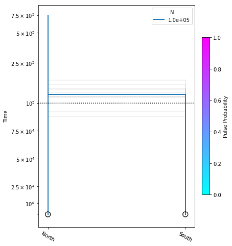
In this figure the thick blue lines indicate the maximum likelihood values estimated under the best model, and the faint lines illustrate results of each of the ten bootstraps.
References
Portik, D. M., Leaché, A. D., Rivera, D., Barej, M. F., Burger, M., Hirschfeld, M., … & Fujita, M. K. (2017). Evaluating mechanisms of diversification in a Guineo‐Congolian tropical forest frog using demographic model selection. Molecular ecology, 26(19), 5245-5263.
Acknowledgements
We relied heavily on the excellent momi2 documentation during the creation of this tutorial.