ipyrad command line tutorial - Part I
This is the first part of the full tutorial for the command line interface (CLI) for ipyrad. In this tutorial we’ll walk through the entire assembly and analysis process. This is meant as a broad introduction to familiarize users with the general workflow, and some of the parameters and terminology. We will use as an example in this tutorial the Anolis data set from the first part of class. However, you can follow along with one of the other example data sets if you like and although your results will vary the procedure will be identical.
If you are new to RADseq analyses, this tutorial will provide a simple overview of how to execute ipyrad, what the data files look like, how to check that your analysis is working, and what the final output formats will be. We will also cover how to run ipyrad on a cluster and to do so efficiently.
Each grey cell in this tutorial indicates a command line interaction.
Lines starting with $ indicate a command that should be executed
in a terminal connected to the Habanero cluster, for example by copying and
pasting the text into your terminal. Elements in code cells surrounded
by angle brackets (e.g.
## Example Code Cell.
## Create an empty file in my home directory called `watdo.txt`
$ touch ~/watdo.txt

## Print "wat" to the screen
$ echo "wat"
wat
Overview of Assembly Steps
Very roughly speaking, ipyrad exists to transform raw data coming off the sequencing instrument into output files that you can use for downstream analysis.
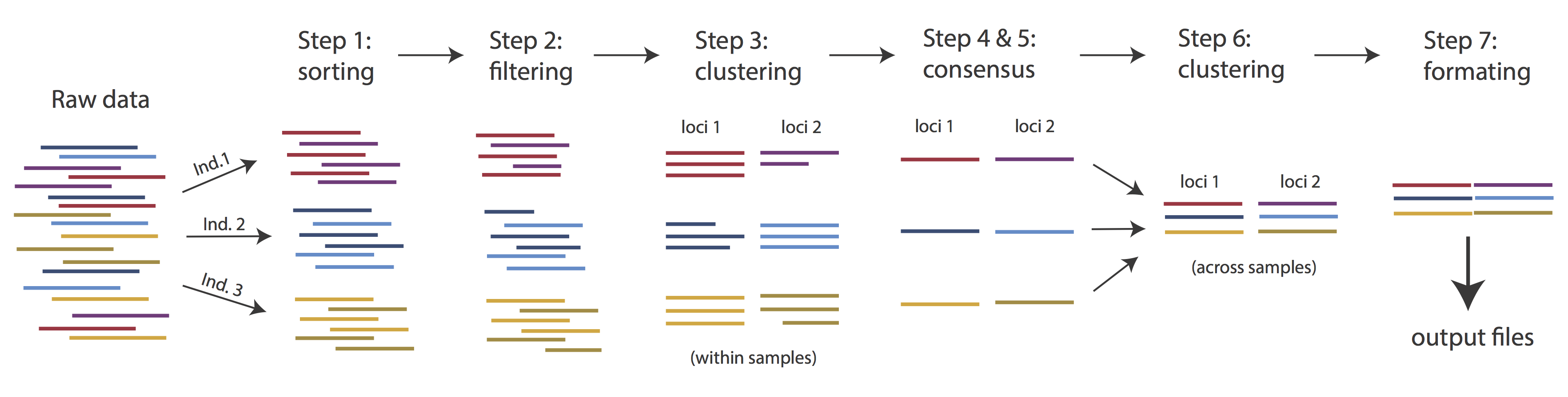
The basic steps of this process are as follows:
- Step 1 - Demultiplex/Load Raw Data
- Step 2 - Trim and Quality Control
- Step 3 - Cluster or reference-map within Samples
- Step 4 - Calculate Error Rate and Heterozygosity
- Step 5 - Call consensus sequences/alleles
- Step 6 - Cluster across Samples
- Step 7 - Apply filters and write output formats
Note on files in the project directory: Assembling RAD-seq type sequence data requires a lot of different steps, and these steps generate a lot of intermediary files. ipyrad organizes these files into directories, and it prepends the name of your assembly to each directory with data that belongs to it. One result of this is that you can have multiple assemblies of the same raw data with different parameter settings and you don’t have to manage all the files yourself! (See Branching assemblies for more info). Another result is that you should not rename or move any of the directories inside your project directory, unless you know what you’re doing or you don’t mind if your assembly breaks.
Getting started
The magic of the Jupyter Hub we’re using for this workshop conceals some of the complexity of working in a real production environment, such as with an HPC system at your home campus. In this case we provide extensive documentation about using ipyrad on HPC systems elsewhere on the RADCamp site.
ipyrad help
To better understand how to use ipyrad, let’s take a look at the help argument. We will use some of the ipyrad arguments in this tutorial (for example: -n, -p, -s, -c, -r). The complete list of optional arguments and their explanation can be accessed with the --help flag:
$ ipyrad --help
usage: ipyrad [-h] [-v] [-r] [-f] [-q] [-d] [-n new] [-p params]
              [-b [branch [branch ...]]] [-m [merge [merge ...]]] [-s steps]
              [-c cores] [-t threading] [--MPI] [--preview]
              [--ipcluster [ipcluster]] [--download [download [download ...]]]

optional arguments:
  -h, --help            show this help message and exit
  -v, --version         show program's version number and exit
  -r, --results         show results summary for Assembly in params.txt and
                        exit
  -f, --force           force overwrite of existing data
  -q, --quiet           do not print to stderror or stdout.
  -d, --debug           print lots more info to ipyrad_log.txt.
  -n new                create new file 'params-{new}.txt' in current
                        directory
  -p params             path to params file for Assembly:
                        params-{assembly_name}.txt
  -b [branch [branch ...]]
                        create a new branch of the Assembly as
                        params-{branch}.txt
  -m [merge [merge ...]]
                        merge all assemblies provided into a new assembly
  -s steps              Set of assembly steps to perform, e.g., -s 123
                        (Default=None)
  -c cores              number of CPU cores to use (Default=0=All)
  -t threading          tune threading of binaries (Default=2)
  --MPI                 connect to parallel CPUs across multiple nodes
  --preview             run ipyrad in preview mode. Subset the input file so
                        it'll runquickly so you can verify everything is
                        working
  --ipcluster [ipcluster]
                        connect to ipcluster profile (default: 'default')
  --download [download [download ...]]
                        download fastq files by accession (e.g., SRP or SRR)

  * Example command-line usage:
    ipyrad -n data                       ## create new file called params-data.txt
    ipyrad -p params-data.txt            ## run ipyrad with settings in params file
    ipyrad -p params-data.txt -s 123     ## run only steps 1-3 of assembly.
    ipyrad -p params-data.txt -s 3 -f    ## run step 3, overwrite existing data.

  * HPC parallelization across 32 cores
    ipyrad -p params-data.txt -s 3 -c 32 --MPI

  * Print results summary
    ipyrad -p params-data.txt -r

  * Branch/Merging Assemblies
    ipyrad -p params-data.txt -b newdata
    ipyrad -m newdata params-1.txt params-2.txt [params-3.txt, ...]

  * Subsample taxa during branching
    ipyrad -p params-data.txt -b newdata taxaKeepList.txt

  * Download sequence data from SRA into directory 'sra-fastqs/'
    ipyrad --download SRP021469 sra-fastqs/

  * Documentation: http://ipyrad.readthedocs.io
Create a new parameters file
ipyrad uses a text file to hold all the parameters for a given assembly.
Start by creating a new parameters file with the -n flag. This flag
requires you to pass in a name for your assembly. In the example we use
simdata but the name can be anything at all. Once you start
analysing your own data you might call your parameters file something
more informative, like the name of your organism and some details on the settings.
# go to our working directory
$ cd ~/work

# create a new params file named 'simdata'
$ ipyrad -n simdata
This will create a file in the current directory called params-simdata.txt. The
params file lists on each line one parameter followed by a ## mark, then the name of the
parameter, and then a short description of its purpose. Lets take a look at it.
$ cat params-simdata.txt
------- ipyrad params file (v.0.7.28)-------------------------------------------
simdata                         ## [0] [assembly_name]: Assembly name. Used to name output directories for assembly steps
./                             ## [1] [project_dir]: Project dir (made in curdir if not present)
                               ## [2] [raw_fastq_path]: Location of raw non-demultiplexed fastq files
                               ## [3] [barcodes_path]: Location of barcodes file
                               ## [4] [sorted_fastq_path]: Location of demultiplexed/sorted fastq files
denovo                         ## [5] [assembly_method]: Assembly method (denovo, reference, denovo+reference, denovo-reference)
                               ## [6] [reference_sequence]: Location of reference sequence file
rad                            ## [7] [datatype]: Datatype (see docs): rad, gbs, ddrad, etc.
TGCAG,                         ## [8] [restriction_overhang]: Restriction overhang (cut1,) or (cut1, cut2)
5                              ## [9] [max_low_qual_bases]: Max low quality base calls (Q<20) in a read
33                             ## [10] [phred_Qscore_offset]: phred Q score offset (33 is default and very standard)
6                              ## [11] [mindepth_statistical]: Min depth for statistical base calling
6                              ## [12] [mindepth_majrule]: Min depth for majority-rule base calling
10000                          ## [13] [maxdepth]: Max cluster depth within samples
0.85                           ## [14] [clust_threshold]: Clustering threshold for de novo assembly
0                              ## [15] [max_barcode_mismatch]: Max number of allowable mismatches in barcodes
0                              ## [16] [filter_adapters]: Filter for adapters/primers (1 or 2=stricter)
35                             ## [17] [filter_min_trim_len]: Min length of reads after adapter trim
2                              ## [18] [max_alleles_consens]: Max alleles per site in consensus sequences
5, 5                           ## [19] [max_Ns_consens]: Max N's (uncalled bases) in consensus (R1, R2)
8, 8                           ## [20] [max_Hs_consens]: Max Hs (heterozygotes) in consensus (R1, R2)
4                              ## [21] [min_samples_locus]: Min # samples per locus for output
20, 20                         ## [22] [max_SNPs_locus]: Max # SNPs per locus (R1, R2)
8, 8                           ## [23] [max_Indels_locus]: Max # of indels per locus (R1, R2)
0.5                            ## [24] [max_shared_Hs_locus]: Max # heterozygous sites per locus (R1, R2)
0, 0, 0, 0                     ## [25] [trim_reads]: Trim raw read edges (R1>, <R1, R2>, <R2) (see docs)
0, 0, 0, 0                     ## [26] [trim_loci]: Trim locus edges (see docs) (R1>, <R1, R2>, <R2)
p, s, v                        ## [27] [output_formats]: Output formats (see docs)
                               ## [28] [pop_assign_file]: Path to population assignment file
In general the defaults are sensible, and we won’t mess with them for now, but there are a few parameters we must change: the path to the raw data, the dataype, the restriction overhang sequence, and the barcodes file.
We will use the nano text editor to modify params-simdata.txt and change
these parameters:
$ nano params-simdata.txt
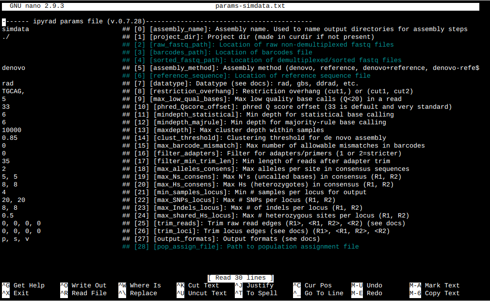
Nano is a command line editor, so you’ll need to use only the arrow keys on the keyboard for navigating around the file. Nano accepts a few special keyboard commands for doing things other than modifying text, and it lists these on the bottom of the frame.
We need to specify where the raw data files are located, the type of data we are using (.e.g., ‘gbs’, ‘rad’, ‘ddrad’, ‘pairddrad), and which enzyme cut site overhangs are expected to be present on the reads. Below are the parameter setings you’ll need to change for the simulated single-end RAD example data:
/home/jovyan/ro-data/ipsimdata/rad_example_R1_.fastq.gz        ## [2] [raw_fastq_path]: Location ofraw non-demultiplexed fastq files
/home/jovyan/ro-data/ipsimdata/rad_example_barcodes.txt        ## [3] [barcodes_path]: Location of barcodes file
rad                            ## [7] [datatype]: Datatype (see docs): rad, gbs, ddrad, etc.
TGCAG,                         ## [8] [restriction_overhang]: Restriction overhang (cut1,) or (cut1, cut2)
After you change these parameters you may save and exit nano by typing CTRL+o (to write Output), and then CTRL+x (to eXit the program).
Note: The
CTRL+xnotation indicates that you should hold down the control key (which is often styled ‘ctrl’ on the keyboard) and then push ‘x’.
Once we start running the analysis ipyrad will create several new
directories to hold the output of each step for this assembly. By
default the new directories are created in the project_dir
directory and use the prefix specified by the assembly_name parameter.
Because we use the default (./) for the project_dir for this tutorial, all these
intermediate directories will be of the form: ~/work/simdata_*,
or the analagous name that you used for your assembly name.
Note: Again, the
./notation indicates the current working directory. You can always view the current working directory with thepwdcommand (print working directory).
Input data format
Before we get started let’s take a look at what the raw data looks like.
Your input data will be in fastQ format, usually ending in .fq,
.fastq, .fq.gz, or .fastq.gz. The file/s may be compressed with
gzip so that they have a .gz ending, but they do not need to be. Lets take
a look at first three reads of one of the simulated data.
$ zcat /home/jovyan/ro-data/ipsimdata/rad_example_R1_.fastq.gz | head -n 12
@lane1_locus0_2G_0_0 1:N:0:
CTCCAATCCTGCAGTTTAACTGTTCAAGTTGGCAAGATCAAGTCGTCCCTAGCCCCCGCGTCCGTTTTTACCTGGTCGCGGTCCCGACCCAGCTGCCCCC
+
BBBBBBBBBBBBBBBBBBBBBBBBBBBBBBBBBBBBBBBBBBBBBBBBBBBBBBBBBBBBBBBBBBBBBBBBBBBBBBBBBBBBBBBBBBBBBBBBBBBB
@lane1_locus0_2G_0_1 1:N:0:
CTCCAATCCTGCAGTTTAACTGTTCAAGTTGGCAAGATCAAGTCGTCCCTAGCCCCCGCGTCCGTTTTTACCTGGTCGCGGTCCCCACCCAGCTGCCCCC
+
BBBBBBBBBBBBBBBBBBBBBBBBBBBBBBBBBBBBBBBBBBBBBBBBBBBBBBBBBBBBBBBBBBBBBBBBBBBBBBBBBBBBBBBBBBBBBBBBBBBB
@lane1_locus0_2G_0_2 1:N:0:
CTCCAATCCTGCAGTTTAACTGTTCAAGTTGGCAAGATCAAGTCGTCCCTAGCCCCCGCGTCCGTTTTTACCTGGTCGCGGTCCCGACCCAGCTGCCCCC
+
BBBBBBBBBBBBBBBBBBBBBBBBBBBBBBBBBBBBBBBBBBBBBBBBBBBBBBBBBBBBBBBBBBBBBBBBBBBBBBBBBBBBBBBBBBBBBBBBBBBB
Exercise for the reader: Can you find and verify the overhang sequence in the simulated data? Hint: It’s not right at the beginning of the sequence, which is where you might expect it to be…. It’s always a good idea to look at your data to check for the cut site. Your first sign of a messy dataset is lots of off target reads, basically stuff that got sequenced that isn’t associated with a restriction enzyme cutsite.
Each read is composed of four lines. The first is the name of the read (its location on the plate). The second line contains the sequence data. The third line is unused. And the fourth line is the quality scores for the base calls. The FASTQ wikipedia page has a good figure depicting the logic behind how quality scores are encoded. Here you can see that the simulated data are generated with uniformly high quality scores. Quality scores in real data are much more all over the place:
@D00656:123:C6P86ANXX:8:2201:3857:34366 1:Y:0:8
TGCATGTTTATTGTCTATGTAAAAGGAAAAGCCATGCTATCAGAGATTGGCCTGGGGGGGGGGGGCAAATACATGAAAAAGGGAAAGGCAAAATG
+
;=11>111>1;EDGB1;=DG1=>1:EGG1>:>11?CE1<>1<1<E1>ED1111:00CC..86DG>....//8CDD/8C/....68..6.:8....
Step 1: Demultiplexing the raw data
Commonly, sequencing facilities will give you one giant .gz file that contains all the reads from all the samples all mixed up together. Step 1 is all about sorting out which reads belong to which samples, so this is where the barcodes file comes in handy. The barcodes file is a simple text file mapping sample names to barcode sequences. Lets look at the simulated barcodes:
$ cat /home/jovyan/ro-data/ipsimdata/rad_example_barcodes.txt
1A_0    CATCATCAT
1B_0    CCAGTGATA
1C_0    TGGCCTAGT
1D_0    GGGAAAAAC
2E_0    GTGGATATC
2F_0    AGAGCCGAG
2G_0    CTCCAATCC
2H_0    CTCACTGCA
3I_0    GGCGCATAC
3J_0    CCTTATGTC
3K_0    ACGTGTGTG
3L_0    TTACTAACA
Here the barcodes are all the same length, but ipyrad can also handle variable length barcodes, and in some cases multiplexed barcodes (3RAD and variants). We can also allow for varying amounts of sequencing error in the barcode in the barcode sequences (parameter 15, max_barcode_mismatch).
Note on step 1: Occasionally sequencing facilities will send back data already demultiplexed to samples. This is totally fine, and is handled natively by ipyrad. In this case you would use the
sorted_fastq_pathin the params file to indiciate the sample fastq.gz files. ipyrad will then scan the samples and load in the raw data.
Now lets run step 1! For the simulated data this will take <10 seconds.
Special Note: In command line mode please be aware to always specify the number of cores with the
-cflag. If you do not specify the number of cores ipyrad assumes you want all of them, which will result in you hogging up all the CPU. We only have 40 cores so everybody has to share!
## -p    the params file we wish to use
## -s    the step to run
## -c    the number of cores to allocate   <-- Important!
$ ipyrad -p params-simdata.txt -s 1 -c 4

 -------------------------------------------------------------
  ipyrad [v.0.7.28]
  Interactive assembly and analysis of RAD-seq data
 -------------------------------------------------------------
  New Assembly: simdata
  establishing parallel connection:
  host compute node: [4 cores] on e305ff77a529

  Step 1: Loading sorted fastq data to Samples
  Step 1: Demultiplexing fastq data to Samples
  [####################] 100%  sorting reads         | 0:00:04
  [####################] 100%  writing/compressing   | 0:00:01
In-depth operations of running an ipyrad step
Any time ipyrad is invoked it performs a few housekeeping operations:
- Load the assembly object - Since this is our first time running any steps we need to initialize our assembly.
- Start the parallel cluster - ipyrad uses a parallelization library called
ipyparallel. Every time we start a step we fire up the parallel clients. This makes your assemblies go smokin’ fast. - Do the work - Actually perform the work of the requested step(s) (in this case demux’ing in sample reads).
- Save, clean up, and exit - Save the state of the assembly and spin down the ipyparallel cluster.
As a convenience ipyrad internally tracks the state of all your steps in your
current assembly, so at any time you can ask for results by invoking the -r flag.
We also use the -p flag to tell it which params file (i.e., which assembly) we
want to print stats for.
## -r fetches informative results from currently executed steps
$ ipyrad -p params-simdata.txt -r
Summary stats of Assembly simdata
------------------------------------------------
      state  reads_raw
1A_0      1      19862
1B_0      1      20043
1C_0      1      20136
1D_0      1      19966
2E_0      1      20017
2F_0      1      19933
2G_0      1      20030
2H_0      1      20199
3I_0      1      19885
3J_0      1      19822
3K_0      1      19965
3L_0      1      20008

Full stats files
------------------------------------------------
step 1: ./simdata_fastqs/s1_demultiplex_stats.txt
step 2: None
step 3: None
step 4: None
step 5: None
step 6: None
step 7: None
If you want to get even more info ipyrad tracks all kinds of wacky stats and saves them to files inside the directories it creates for each step. For instance to see full stats for step 1 (the wackyness of the step 1 stats at this point isn’t very interesting, but we’ll see stats for later steps are more verbose):
$ cat simdata_fastqs/s1_demultiplex_stats.txt
raw_file                               total_reads    cut_found  bar_matched
rad_example_R1_.fastq                       239866       239866       239866

sample_name                            total_reads
1A_0                                         19862
1B_0                                         20043
1C_0                                         20136
1D_0                                         19966
2E_0                                         20017
2F_0                                         19933
2G_0                                         20030
2H_0                                         20199
3I_0                                         19885
3J_0                                         19822
3K_0                                         19965
3L_0                                         20008

sample_name                               true_bar       obs_bar     N_records
1A_0                                     CATCATCAT     CATCATCAT         19862
1B_0                                     CCAGTGATA     CCAGTGATA         20043
1C_0                                     TGGCCTAGT     TGGCCTAGT         20136
1D_0                                     GGGAAAAAC     GGGAAAAAC         19966
2E_0                                     GTGGATATC     GTGGATATC         20017
2F_0                                     AGAGCCGAG     AGAGCCGAG         19933
2G_0                                     CTCCAATCC     CTCCAATCC         20030
2H_0                                     CTCACTGCA     CTCACTGCA         20199
3I_0                                     GGCGCATAC     GGCGCATAC         19885
3J_0                                     CCTTATGTC     CCTTATGTC         19822
3K_0                                     ACGTGTGTG     ACGTGTGTG         19965
3L_0                                     TTACTAACA     TTACTAACA         20008
no_match                                         _            _            0
Another early indicator of trouble is if you have a ton of reads that are no_match.
This means maybe your barcodes file is wrong, or maybe your library prep went poorly. Here,
with the simulated data we have no unmatched barcodes, because, well, it’s simulated.
Step 2: Filter reads
This step filters reads based on quality scores and maximum number of uncalled bases, and can be used to detect Illumina adapters in your reads, which is sometimes a problem under a couple different library prep scenarios. Since it’s not atypical to have adapter contamination issues and to have a little noise toward the distal end of the reads lets imagine this is true of the simulated data, and we’ll try to account for this by trimming reads to 90bp and using aggressive adapter filtering.
Edit your params file again with nano:
nano params-simdata.txt
and change the following two parameter settings:
2                               ## [16] [filter_adapters]: Filter for adapters/primers (1 or 2=stricter)
0, 90, 0, 0                     ## [25] [trim_reads]: Trim raw read edges (R1>, <R1, R2>, <R2) (see docs)
Note: Saving and quitting from
nano:CTRL+othenCTRL+x
$ ipyrad -p params-simdata.txt -s 2 -c 4
 -------------------------------------------------------------
  ipyrad [v.0.7.28]
  Interactive assembly and analysis of RAD-seq data
 -------------------------------------------------------------
  loading Assembly: simdata
  from saved path: ~/work/simdata.json
  establishing parallel connection:
  host compute node: [4 cores] on darwin

  Step 2: Filtering reads
  [####################] 100%  processing reads      | 0:00:12
The filtered files are written to a new directory called simdata_edits. Again,
you can look at the results output by this step and also some handy stats tracked
for this assembly.
## View the output of step 2
$ cat simdata_edits/s2_rawedit_stats.txt
      reads_raw  trim_adapter_bp_read1  trim_quality_bp_read1  reads_filtered_by_Ns  reads_filtered_by_minlen  reads_passed_filter
1A_0      19862                    360                      0                     0                         0  19862
1B_0      20043                    362                      0                     0                         0  20043
1C_0      20136                    349                      0                     0                         0  20136
1D_0      19966                    404                      0                     0                         0  19966
2E_0      20017                    394                      0                     0                         0  20017
2F_0      19933                    376                      0                     0                         0  19933
2G_0      20030                    381                      0                     0                         0  20030
2H_0      20199                    386                      0                     0                         1  20198
3I_0      19885                    372                      0                     0                         0  19885
3J_0      19822                    381                      0                     0                         0  19822
3K_0      19965                    382                      0                     0                         0  19965
3L_0      20008                    424                      0                     0                         0  20008
It’s a little boring, the reads are too clean. Here is an example of something
like you’d see from real data (this is the Anolis dataset). Notice the reads_passed_filter
value. This dataset is decent, as you can see we’re losing < 10% of the reads per sample,
mostly due to the minimum length cutoff.
                   reads_raw  trim_adapter_bp_read1  trim_quality_bp_read1  reads_filtered_by_Ns  reads_filtered_by_minlen  reads_passed_filter
punc_IBSPCRIB0361     250000                 108761                 160210                    66                     12415               237519
punc_ICST764          250000                 107320                 178463                    68                     13117               236815
punc_JFT773           250000                 110684                 190803                    46                      9852               240102
punc_MTR05978         250000                 102932                 144773                    54                     12242               237704
punc_MTR17744         250000                 103394                 211363                    55                      9549               240396
punc_MTR21545         250000                 119191                 161709                    63                     21972               227965
punc_MTR34414         250000                 109207                 193401                    54                     16372               233574
punc_MTRX1468         250000                 119746                 134069                    45                     19052               230903
punc_MTRX1478         250000                 116009                 184189                    53                     16549               233398
punc_MUFAL9635        250000                 114492                 182877                    61                     18071               231868
## Get current stats including # raw reads and # reads after filtering.
$ ipyrad -p params-simdata.txt -r
You might also take a closer look at the filtered reads:
$ zcat simdata_edits/1A_0.trimmed_R1_.fastq.gz | head -n 12
@lane1_locus0_1A_0_0 1:N:0:
TGCAGTTTAACTGTTCAAGTTGGCAAGATCAAGTCGTCCCTAGCCCCCGCGTCCGTTTTTACCTGGTCGCGGTCCCGACCCAGCTGCCCC
+
BBBBBBBBBBBBBBBBBBBBBBBBBBBBBBBBBBBBBBBBBBBBBBBBBBBBBBBBBBBBBBBBBBBBBBBBBBBBBBBBBBBBBBBBBB
@lane1_locus0_1A_0_1 1:N:0:
TGCAGTTTAACTGTTCAAGTTGGCAAGATCAAGTCGTCCCTAGCCCCCGCGTCCGTTTTTACCTGGTCGCGGTCCCGACCCAGCTGCCCC
+
BBBBBBBBBBBBBBBBBBBBBBBBBBBBBBBBBBBBBBBBBBBBBBBBBBBBBBBBBBBBBBBBBBBBBBBBBBBBBBBBBBBBBBBBBB
@lane1_locus0_1A_0_2 1:N:0:
TGCAGTTTAACTGTTCAAGTTGGCAAGATCAAGTCGTCCCTAGCCCCCGCGTCCGTTTTTACCTGGTCGCGGTCCCGACCCAGCTGCCCC
+
BBBBBBBBBBBBBBBBBBBBBBBBBBBBBBBBBBBBBBBBBBBBBBBBBBBBBBBBBBBBBBBBBBBBBBBBBBBBBBBBBBBBBBBBBB
Since the adapter content of the simulated data is effectively 0, the net effect of step 2 is that the reads have been trimmed to 90bp. This isn’t necessary here, but it provides a good example since real data typically will need trimming.
Step 3: clustering within-samples
Step 3 de-replicates and then clusters reads within each sample by the
set clustering threshold and then writes the clusters to new files in a
directory called simdata_clust_0.85. Intuitively we are trying to
identify all the reads that map to the same locus within each sample.
The clustering threshold specifies the minimum percentage of sequence
similarity below which we will consider two reads to have come from
different loci.
The true name of this output directory will be dictated by the value you
set for the clust_threshold parameter in the params file. This makes it
very easy to test different clustering thresholds, and keep the different
runs organized (since you will have for example simdata_clust_0.85 and
simdata_clust_0.9).
You can see the default value is 0.85, so our default directory is named accordingly. This value dictates the percentage of sequence similarity that reads must have in order to be considered reads at the same locus. You’ll more than likely want to experiment with this value, but 0.85 is a reliable default, balancing over-splitting of loci vs over-lumping. Don’t mess with this until you feel comfortable with the overall workflow, and also until you’ve learned about Branching assemblies (which we will get to later this afternoon).
There have been many papers written comparing how results of assemblies vary depending on the clustering threshold. In general, my advice is to use a value between about .82 and .95. Within this region results typically do not vary too significantly, whereas above .95 you will oversplit loci and recover fewer SNPs.
It’s also possible to incorporate information from a reference genome to improve clustering at this step, if such a resources is available for your organism (or one that is relatively closely related). We will not cover reference based assemblies in this workshop, but you can refer to the ipyrad documentation for more information.
Note on performance: Steps 3 and 6 generally take considerably longer than any of the other steps, due to the resource intensive clustering and alignment phases. These can take on the order of 10-100x as long as the next longest running step. This depends heavily on the number of samples in your dataset, the number of cores on your computer, the length(s) of your reads, and the “messiness” of your data in terms of the number of unique loci present (this can vary from a few thousand to many millions).
Now lets run step 3:
$ ipyrad -p params-simdata.txt -s 3 -c 4
 -------------------------------------------------------------
  ipyrad [v.0.7.28]
  Interactive assembly and analysis of RAD-seq data
 -------------------------------------------------------------
  loading Assembly: simdata
  from saved path: ~/work/simdata.json
  establishing parallel connection:
  host compute node: [4 cores] on e305ff77a529

  Step 3: Clustering/Mapping reads within samples
  [####################] 100% 0:00:01 | concatenating
  [####################] 100% 0:00:01 | dereplicating
  [####################] 100% 0:00:00 | clustering/mapping
  [####################] 100% 0:00:00 | building clusters
  [####################] 100% 0:00:00 | chunking clusters
  [####################] 100% 0:00:03 | aligning clusters
  [####################] 100% 0:00:00 | concat clusters
  [####################] 100% 0:00:00 | calc cluster stats
In-depth operations of step 3:
- concatenating - Concatenate files from merged assemblies
- dereplicating - Merge all identical reads
- clustering - Find reads matching by sequence similarity threshold
- building clusters - Group similar reads into clusters
- chunking - Subsample cluster files to improve performance of alignment step
- aligning - Align all clusters
- concatenating - Gather chunked clusters into one full file of aligned clusters
- calc cluster stats - Just as it says!
Again we can examine the results. The stats output tells you how many clusters were found (‘clusters_total’), and the number of clusters that pass the mindepth thresholds (‘clusters_hidepth’). We go into more detail about mindepth settings in some of the advanced tutorials but for now all you need to know is that by default step 3 will filter out clusters that only have a handful of reads on the assumption that it will be difficult to accurately call bases at such low depth.
$ ipyrad -p params-simdata.txt -r
Summary stats of Assembly simdata
------------------------------------------------
      state  reads_raw  reads_passed_filter  clusters_total  clusters_hidepth
1A_0      3      19862                19862            1000              1000
1B_0      3      20043                20043            1000              1000
1C_0      3      20136                20136            1000              1000
1D_0      3      19966                19966            1000              1000
2E_0      3      20017                20017            1000              1000
2F_0      3      19933                19933            1000              1000
2G_0      3      20030                20030            1000              1000
2H_0      3      20199                20198            1000              1000
3I_0      3      19885                19885            1000              1000
3J_0      3      19822                19822            1000              1000
3K_0      3      19965                19965            1000              1000
3L_0      3      20008                20008            1000              1000


Full stats files
------------------------------------------------
step 1: ./simdata_fastqs/s1_demultiplex_stats.txt
step 2: ./simdata_edits/s2_rawedit_stats.txt
step 3: ./simdata_clust_0.85/s3_cluster_stats.txt
Again, the final output of step 3 is dereplicated, clustered files for
each sample in ./simdata_0.85/. You can get a feel for what
this looks like by examining a portion of one of the files.
## Same as above, `zcat` unzips and prints to the screen and
## `head -n 24` means just show me the first 24 lines.
$  zcat simdata_clust_0.85/1A_0.clustS.gz | head -n 24
009149cc23d2367f21b67ac0060d9f2f;size=18;*
TGCAGATAAATCAAACTGCAGCTTGATATGGGCTTCGACCCAGTGGTGGTAGCCTCTCTCTCCCAGTATAACCTCGACCCCAAAATCGCA
d498af3d4575b871de6d5a7f239279ea;size=1;+
TGCAGATAAATCAAACTGCAGCTTGATATGGGCTTCGACCCAGTGGTGGTAGCCTCTCTCTCCCAGTATAACCTCGACCCCAAAATCGCT
b71555537ed7f88329fda094cc6cef8a;size=1;+
TGCAGATAAATCAAACTGCAGCTTGATATGGGCTTCGACCCAGTGGTGGTAGCGTCTCTCTCCCAGTATAACCTCGACCCCAAAATCGCA
//
//
00f1daaa8dd241bd72db91aa62b31bb4;size=8;*
TGCAGGGGTTAGGCGTATCTGCCAAAGATTCTTCGATCGTGATGATTCTAGACGACAATACACCTGATGCTTCTCGCATGCATAGCAATG
6780649efadfc8c182cfd2af7071316b;size=8;+
TGCAGGGGTTAGGCGTATCTGCCAAAGATTCTTCGATCGTGATGATTCTAGAGGACAATACACCTGATGCTTCTCGCATGCATAGCAATG
23a7b43b7f5008017574400c460982dc;size=1;+
TGCAGGGGTTAGGCGTATCTTCCAAAGATTCTTCGATCGTGATGATTCTAGACGACAATACACCTGATGCTTCTCGCATGCATAGCAATG
e6830f9099df558397f0fd28bf9568b6;size=1;+
TGCAGGGGTTAGGCGTATCTGCCAAAGATTCTTCGATCGTGATGATTCTAGACGATAATACACCTGATGCTTCTCGCATGCATAGCAATG
//
//
013b4e939c785d94369ea933f7f98f0c;size=18;*
TGCAGATACTTCGCCCGGTTCTCCATACCCCATTCTTTGCTGCTTCTTCTGAGCGCACTCGACCTATGCCTAGTCGCACCTCGCATATTT
a7e612c565f1d70f054864759b58205f;size=1;+
TGCAGATACTTCGCCCGGTTCTCCATACCCCATTCTTTGCTGCTTCTTCTGAGCGCACTCGACCTATGCCTAGTCCCACCTCGCATATTT
//
//
Reads that are sufficiently similar (based on the above sequence similarity threshold) are grouped together in clusters separated by “//”. For the second cluster above this is probably heterozygous with some sequencing error, and the first and third clusters are probably homozygous. Again, the simulated data is too clean to get a real picture of how tricky real data can be. Looking again at the Anolis data:
000e3bb624e3bd7e91b47238b7314dc6;size=4;*
TGCATATCACAAGAGAAGAAAGCCACTAATTAAGGGGAAAAGAAAAGCCTCTGATATAGCTCCGATATATCATGC-
75e462e101383cca3db0c02fca80b37a;size=2;-
-GCATATCACAAGAGAAGAAAGCCACTAATTAAGGGGAAAAGAAAAGCCTCTGATATAGCTCCGATATATCATGCA
//
//
001236a2310c39a3a16d96c4c6c48df1;size=4;*
TGCATCTCTTTGGGCTGTTGCTTGGTGGCACACCATGCTGCTTTCTCCTCACTTTTTCTCTCTTTTCCTGAGACT------------------------------
4644056dca0546a270ba897b018624b4;size=2;-
------------------------------CACCATGCTGCTTTCTCCTCACTTTTTCTCTCTTTTCCTGAGACTGAGCCAGGGACAGCGGCTGAGGAGGATGCA
5412b772ec0429af178caf6040d2af30;size=1;+
TGCATTTCTTTGGGCTGTTGCTTGGTGGCACACCATGCTGCTTTCTCCTCACTTTTTCTCTCTTTTCCTGAGACT------------------------------
//
//
Are there truly two alleles (heterozygote) for each of these loci? Are they homozygous with lots of sequencing errors, or a heterozygote with few reads for one of the alleles?
Thankfully, untangling this mess is what step 4 is all about.