ipyrad command line tutorial - Part I
This is the first part of the full tutorial for the command line interface (CLI) for ipyrad. In this tutorial we’ll walk through the entire assembly and analysis process. This is meant as a broad introduction to familiarize users with the general workflow, and some of the parameters and terminology. We will use simulated paired-end ddRAD data as an example in this tutorial, however, you can follow along with one of the other example datasets if you like and although your results will vary the procedure will be identical.
If you are new to RADseq analyses, this tutorial will provide a simple overview of how to execute ipyrad, what the data files look like, how to check that your analysis is working, and what the final output formats will be. We will also cover how to run ipyrad on a cluster and how to do so efficiently.
Each grey cell in this tutorial indicates a command line interaction.
Lines starting with $ indicate a command that should be executed
in a terminal connected to the Habanero cluster, for example by copying and
pasting the text into your terminal. Elements in code cells surrounded
by angle brackets (e.g.
## Example Code Cell.
## Create an empty file in my home directory called `watdo.txt`
$ touch ~/watdo.txt

## Print "wat" to the screen
$ echo "wat"
wat
Overview of Assembly Steps
Very roughly speaking, ipyrad exists to transform raw data coming off the sequencing instrument into output files that you can use for downstream analysis.
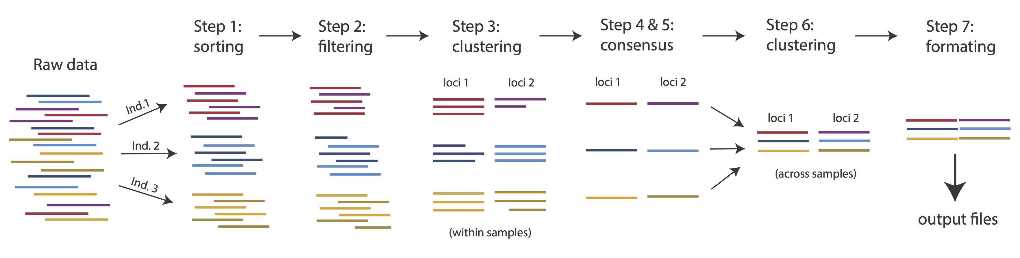
The basic steps of this process are as follows:
- Step 1 - Demultiplex/Load Raw Data
- Step 2 - Trim and Quality Control
- Step 3 - Cluster or reference-map within Samples
- Step 4 - Calculate Error Rate and Heterozygosity
- Step 5 - Call consensus sequences/alleles
- Step 6 - Cluster across Samples
- Step 7 - Apply filters and write output formats
Note on files in the project directory: Assembling RADseq type sequence data requires a lot of different steps, and these steps generate a lot of intermediary files. ipyrad organizes these files into directories, and it prepends the name of your assembly to each directory with data that belongs to it. One result of this is that you can have multiple assemblies of the same raw data with different parameter settings and you don’t have to manage all the files yourself! (See Branching assemblies for more info). Another result is that you should not rename or move any of the directories inside your project directory, unless you know what you’re doing or you don’t mind if your assembly breaks.
Getting Started
We will be running through the assembly of simulated data on a binder instance, so if you haven’t already, please launch the ipyrad repo, and open a New>Terminal.
ipyrad help
To better understand how to use ipyrad, let’s take a look at the help argument. We will use some of the ipyrad arguments in this tutorial (for example: -n, -p, -s, -c, -r). But, the complete list of optional arguments and their explanation is below.
$ ipyrad -h

usage: ipyrad [-h] [-v] [-r] [-f] [-q] [-d] [-n NEW] [-p PARAMS] [-s STEPS] [-b [BRANCH [BRANCH ...]]]
              [-m [MERGE [MERGE ...]]] [-c cores] [-t threading] [--MPI] [--ipcluster [IPCLUSTER]]
              [--download [DOWNLOAD [DOWNLOAD ...]]]

optional arguments:
  -h, --help            show this help message and exit
  -v, --version         show program's version number and exit
  -r, --results         show results summary for Assembly in params.txt and exit
  -f, --force           force overwrite of existing data
  -q, --quiet           do not print to stderror or stdout.
  -d, --debug           print lots more info to ipyrad_log.txt.
  -n NEW                create new file 'params-{new}.txt' in current directory
  -p PARAMS             path to params file for Assembly: params-{assembly_name}.txt
  -s STEPS              Set of assembly steps to run, e.g., -s 123
  -b [BRANCH [BRANCH ...]]
                        create new branch of Assembly as params-{branch}.txt, and can be used to drop samples from
                        Assembly.
  -m [MERGE [MERGE ...]]
                        merge multiple Assemblies into one joint Assembly, and can be used to merge Samples into one
                        Sample.
  -c cores              number of CPU cores to use (Default=0=All)
  -t threading          tune threading of multi-threaded binaries (Default=2)
  --MPI                 connect to parallel CPUs across multiple nodes
  --ipcluster [IPCLUSTER]
                        connect to running ipcluster, enter profile name or profile='default'
  --download [DOWNLOAD [DOWNLOAD ...]]
                        download fastq files by accession (e.g., SRP or SRR)

  * Example command-line usage:
    ipyrad -n data                       ## create new file called params-data.txt
    ipyrad -p params-data.txt -s 123     ## run only steps 1-3 of assembly.
    ipyrad -p params-data.txt -s 3 -f    ## run step 3, overwrite existing data.

  * HPC parallelization across 32 cores
    ipyrad -p params-data.txt -s 3 -c 32 --MPI

  * Print results summary
    ipyrad -p params-data.txt -r

  * Branch/Merging Assemblies
    ipyrad -p params-data.txt -b newdata
    ipyrad -m newdata params-1.txt params-2.txt [params-3.txt, ...]

  * Subsample taxa during branching
    ipyrad -p params-data.txt -b newdata taxaKeepList.txt

  * Download sequence data from SRA into directory 'sra-fastqs/'
    ipyrad --download SRP021469 sra-fastqs/

  * Documentation: http://ipyrad.readthedocs.io
Create a new parameters file
ipyrad uses a text file to hold all the parameters for a given assembly.
Start by creating a new parameters file with the -n flag. This flag
requires you to pass in a name for your assembly. In the example we use
peddrad but the name can be anything at all. Once you start
analysing your own data you might call your parameters file something
more informative, like the name of your organism and some details on the
settings.
# First, make sure you're in your workshop directory
$ cd ~/ipyrad-workshop

# Unpack the simulated data which is included in the ipyrad github repo
# `tar` is a program for reading and writing archive files, somewhat like zip
#   -x eXtract from an archive
#   -z unZip before extracting
#   -f read from the File
$ tar -xzf ~/tests/ipsimdata.tar.gz

# Take a look at what we just unpacked
$ ls ipsimdata
gbs_example_barcodes.txt         pairddrad_example_R2_.fastq.gz         pairgbs_wmerge_example_genome.fa
gbs_example_genome.fa            pairddrad_wmerge_example_barcodes.txt  pairgbs_wmerge_example_R1_.fastq.gz
gbs_example_R1_.fastq.gz         pairddrad_wmerge_example_genome.fa     pairgbs_wmerge_example_R2_.fastq.gz
pairddrad_example_barcodes.txt   pairddrad_wmerge_example_R1_.fastq.gz  rad_example_barcodes.txt
pairddrad_example_genome.fa      pairddrad_wmerge_example_R2_.fastq.gz  rad_example_genome.fa
pairddrad_example_genome.fa.fai  pairgbs_example_barcodes.txt           rad_example_genome.fa.fai
pairddrad_example_genome.fa.sma  pairgbs_example_R1_.fastq.gz           rad_example_genome.fa.sma
pairddrad_example_genome.fa.smi  pairgbs_example_R2_.fastq.gz           rad_example_genome.fa.smi
pairddrad_example_R1_.fastq.gz   pairgbs_wmerge_example_barcodes.txt    rad_example_R1_.fastq.gz
You can see that we provide a bunch of different example datasets, as well as
toy genomes for testing different assembly methods. For now we’ll go forward
with the pairddrad example dataset.
# Now create a new params file named 'peddrad'
$ ipyrad -n peddrad
This will create a file in the current directory called params-peddrad.txt.
The params file lists on each line one parameter followed by a ## mark,
then the name of the parameter, and then a short description of its purpose.
Lets take a look at it.
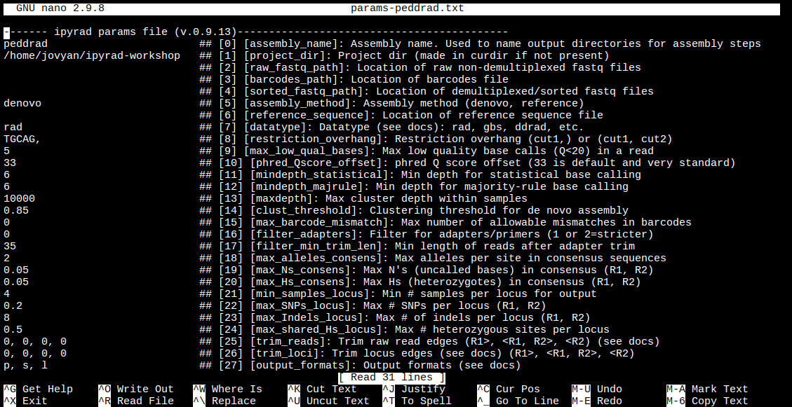
$ cat params-peddrad.txt
------- ipyrad params file (v.0.9.13)-------------------------------------------
peddrad                        ## [0] [assembly_name]: Assembly name. Used to name output directories for assembly steps
/home/jovyan/ipyrad-workshop   ## [1] [project_dir]: Project dir (made in curdir if not present)
                               ## [2] [raw_fastq_path]: Location of raw non-demultiplexed fastq files
                               ## [3] [barcodes_path]: Location of barcodes file
                               ## [4] [sorted_fastq_path]: Location of demultiplexed/sorted fastq files
denovo                         ## [5] [assembly_method]: Assembly method (denovo, reference)
                               ## [6] [reference_sequence]: Location of reference sequence file
rad                            ## [7] [datatype]: Datatype (see docs): rad, gbs, ddrad, etc.
TGCAG,                         ## [8] [restriction_overhang]: Restriction overhang (cut1,) or (cut1, cut2)
5                              ## [9] [max_low_qual_bases]: Max low quality base calls (Q<20) in a read
33                             ## [10] [phred_Qscore_offset]: phred Q score offset (33 is default and very standard)
6                              ## [11] [mindepth_statistical]: Min depth for statistical base calling
6                              ## [12] [mindepth_majrule]: Min depth for majority-rule base calling
10000                          ## [13] [maxdepth]: Max cluster depth within samples
0.85                           ## [14] [clust_threshold]: Clustering threshold for de novo assembly
0                              ## [15] [max_barcode_mismatch]: Max number of allowable mismatches in barcodes
0                              ## [16] [filter_adapters]: Filter for adapters/primers (1 or 2=stricter)
35                             ## [17] [filter_min_trim_len]: Min length of reads after adapter trim
2                              ## [18] [max_alleles_consens]: Max alleles per site in consensus sequences
0.05                           ## [19] [max_Ns_consens]: Max N's (uncalled bases) in consensus (R1, R2)
0.05                           ## [20] [max_Hs_consens]: Max Hs (heterozygotes) in consensus (R1, R2)
4                              ## [21] [min_samples_locus]: Min # samples per locus for output
0.2                            ## [22] [max_SNPs_locus]: Max # SNPs per locus (R1, R2)
8                              ## [23] [max_Indels_locus]: Max # of indels per locus (R1, R2)
0.5                            ## [24] [max_shared_Hs_locus]: Max # heterozygous sites per locus
0, 0, 0, 0                     ## [25] [trim_reads]: Trim raw read edges (R1>, <R1, R2>, <R2) (see docs)
0, 0, 0, 0                     ## [26] [trim_loci]: Trim locus edges (see docs) (R1>, <R1, R2>, <R2)
p, s, l                        ## [27] [output_formats]: Output formats (see docs)
                               ## [28] [pop_assign_file]: Path to population assignment file
                               ## [29] [reference_as_filter]: Reads mapped to this reference are removed in step 3
In general the defaults are sensible, and we won’t mess with them for now, but there are a few parameters we must change: the path to the raw data and the barcodes file, the dataype, and the restriction overhang sequence(s).
We will use the nano text editor to modify params-peddrad.txt and change
these parameters:
# First we have to install nano. You will have to do this every time you
# launch a new binder, since it's not part of the ipyrad rep
$ conda install nano -y

# Change one stupid default setting. This is annoying <sorry!>
$ echo "set nowrap" > ~/.nanorc

# Now you can edit the params file
$ nano params-peddrad.txt
Nano is a command line editor, so you’ll need to use only the arrow keys on the keyboard for navigating around the file. Nano accepts a few special keyboard commands for doing things other than modifying text, and it lists these on the bottom of the frame.
We need to specify where the raw data files are located, the type of data we are using (.e.g., ‘gbs’, ‘rad’, ‘ddrad’, ‘pairddrad), and which enzyme cut site overhangs are expected to be present on the reads. Change the following lines in your params files to look like this:
ipsimdata/pairddrad_example_R*.fastq.gz     ## [2] [raw_fastq_path]: Location of raw non-demultiplexed fastq files
ipsimdata/pairddrad_example_barcodes.txt    ## [3] [barcodes_path]: Location of barcodes file
pairddrad                                   ## [7] [datatype]: Datatype (see docs): rad, gbs, ddrad, etc.
TGCAG, CGG                                  ## [8] [restriction_overhang]: Restriction overhang (cut1,) or (cut1, cut2)
After you change these parameters you may save and exit nano by typing CTRL+o (to write Output), and then CTRL+x (to eXit the program).
Note: The
CTRL+xnotation indicates that you should hold down the control key (which is often styled ‘ctrl’ on the keyboard) and then push ‘x’.
Once we start running the analysis ipyrad will create several new directories to
hold the output of each step for this assembly. By default the new directories
are created in the project_dir directory and use the prefix specified by the
assembly_name parameter. For this example assembly all the intermediate
directories will be of the form: ~/ipyrad-workshop/peddrad_*.
Note: Again, the
~notation indicates a shortcut for the user home directory, in this case/home/jovyan.
Input data format
Before we get started, let’s take a look at what the raw data looks like. Remember that you can use zcat and head to do this.
## zcat: unZip and conCATenate the file to the screen
## head -n 20: Just take the first 20 lines of input

$ zcat ipsimdata/pairddrad_example_R1_.fastq.gz | head -n 20
@lane1_locus0_2G_0_0 1:N:0:
CTCCAATCCTGCAGTTTAACTGTTCAAGTTGGCAAGATCAAGTCGTCCCTAGCCCCCGCGTCCGTTTTTACCTGGTCGCGGTCCCGACCCAGCTGCCCCC
+
BBBBBBBBBBBBBBBBBBBBBBBBBBBBBBBBBBBBBBBBBBBBBBBBBBBBBBBBBBBBBBBBBBBBBBBBBBBBBBBBBBBBBBBBBBBBBBBBBBBB
@lane1_locus0_2G_0_1 1:N:0:
CTCCAATCCTGCAGTTTAACTGTTCAAGTTGGCAAGATCAAGTCGTCCCTAGCCCCCGCGTCCGTTTTTACCTGGTCGCGGTCCCGACCCAGCTGCCCCC
+
BBBBBBBBBBBBBBBBBBBBBBBBBBBBBBBBBBBBBBBBBBBBBBBBBBBBBBBBBBBBBBBBBBBBBBBBBBBBBBBBBBBBBBBBBBBBBBBBBBBB
@lane1_locus0_2G_0_2 1:N:0:
CTCCAATCCTGCAGTTTAACTGTTCAAGTTGGCAAGATCAAGTCGTCCCTAGCCCCCGCGTCCGTTTTTACCTGGTCGCGGTCCCGACCCAGCTGCCCCC
+
BBBBBBBBBBBBBBBBBBBBBBBBBBBBBBBBBBBBBBBBBBBBBBBBBBBBBBBBBBBBBBBBBBBBBBBBBBBBBBBBBBBBBBBBBBBBBBBBBBBB
@lane1_locus0_2G_0_3 1:N:0:
CTCCAATCCTGCAGTTTAACTGTTCAAGTTGGCAAGATCAAGTCGTCCCTAGCCCCCGCGTCCGTTTTTACCTGGTCGCGGTCCCGACCCAGCTGCCCCC
+
BBBBBBBBBBBBBBBBBBBBBBBBBBBBBBBBBBBBBBBBBBBBBBBBBBBBBBBBBBBBBBBBBBBBBBBBBBBBBBBBBBBBBBBBBBBBBBBBBBBB
@lane1_locus0_2G_0_4 1:N:0:
CTCCAATCCTGCAGTTTAACTGTTCAAGTTGGCAAGATCAAGTCGTCCCTAGCCCCCGCGTCCGTTTTTACCTGGTCGCGGTCCCGACCCAGCTGCCCCC
+
BBBBBBBBBBBBBBBBBBBBBBBBBBBBBBBBBBBBBBBBBBBBBBBBBBBBBBBBBBBBBBBBBBBBBBBBBBBBBBBBBBBBBBBBBBBBBBBBBBBB
The simulated data are 100bp paired-end reads generated as ddRAD, meaning there will be two overhang sequences. In this case the ‘rare’ cutter leaves the TGCAT overhang. Can you find this sequence in the raw data? What’s going on with that other stuff at the beginning of each read?
Step 1: Demultiplexing the raw data
Since the raw data is still just a huge pile of reads, we need to split it up
and assign each read to the sample it came from. This will create a new
directory called peddrad_fastqs with one .gz file per sample.
Note on step 1: Sometimes, rather than returning the raw data, sequencing facilities will give the data pre-demultiplexed to samples. This situation only slightly modifies step 1, and does not modify further steps, so we will refer you to the full ipyrad tutorial for guidance in this case.
Now lets run step 1! For the simulated data this will take just a few moments.
Special Note: It’s good practice to specify the number of cores with the
-cflag. If you do not specify the number of cores ipyrad assumes you want all of them. Binder instances run on 1 core, so we will specify-c 1for all ipyrad assembly steps.
## -p    the params file we wish to use
## -s    the step to run
## -c    run on 1 core
$ ipyrad -p params-peddrad.txt -s 1 -c 1

 -------------------------------------------------------------
  ipyrad [v.0.9.13]
  Interactive assembly and analysis of RAD-seq data
 -------------------------------------------------------------
  Parallel connection | jupyter-dereneaton-2dipyrad-2d975c3axu: 1 cores

  Step 1: Demultiplexing fastq data to Samples
  [####################] 100% 0:00:09 | sorting reads
  [####################] 100% 0:00:05 | writing/compressing

  Parallel connection closed.
In-depth operations of running an ipyrad step
Any time ipyrad is invoked it performs a few housekeeping operations:
- Load the assembly object - Since this is our first time running any steps we need to initialize our assembly.
- Start the parallel cluster - ipyrad uses a parallelization library called ipyparallel. Every time we start a step we fire up the parallel clients. This makes your assemblies go smokin’ fast.
- Do the work - Actually perform the work of the requested step(s) (in this case demultiplexing reads to samples).
- Save, clean up, and exit - Save the state of the assembly, and spin down the ipyparallel cluster.
As a convenience ipyrad internally tracks the state of all your steps in your
current assembly, so at any time you can ask for results by invoking the -r
flag. We also use the -p argument to tell it which params file (i.e., which
assembly) we want it to print stats for.
## -r fetches informative results from currently executed steps
$ ipyrad -p params-peddrad.txt -r
  loading Assembly: peddrad
  from saved path: ~/ipyrad-workshop/peddrad.json

Summary stats of Assembly peddrad
------------------------------------------------
      state  reads_raw
1A_0      1      19835
1B_0      1      20071
1C_0      1      19969
1D_0      1      20082
2E_0      1      20004
2F_0      1      19899
2G_0      1      19928
2H_0      1      20110
3I_0      1      20078
3J_0      1      19965
3K_0      1      19846
3L_0      1      20025


Full stats files
------------------------------------------------
step 1: ./peddrad_fastqs/s1_demultiplex_stats.txt
step 2: None
step 3: None
step 4: None
step 5: None
step 6: None
step 7: None
If you want to get even more info, ipyrad tracks all kinds of wacky stats and saves them to a file inside the directories it creates for each step. For instance, to see full stats for step 1 (the wackyness of the step 1 stats at this point isn’t very interesting, but we’ll see stats for later steps are more verbose):
$ cat peddrad_fastqs/s1_demultiplex_stats.txt
raw_file                               total_reads    cut_found  bar_matched
pairddrad_example_R1_.fastq                 239812       239812       239812
pairddrad_example_R2_.fastq                 239812       239812       239812

sample_name                            total_reads
1A_0                                         19835
1B_0                                         20071
1C_0                                         19969
1D_0                                         20082
2E_0                                         20004
2F_0                                         19899
2G_0                                         19928
2H_0                                         20110
3I_0                                         20078
3J_0                                         19965
3K_0                                         19846
3L_0                                         20025

sample_name                               true_bar       obs_bar     N_records
1A_0                                     CATCATCAT     CATCATCAT         19835
1B_0                                     CCAGTGATA     CCAGTGATA         20071
1C_0                                     TGGCCTAGT     TGGCCTAGT         19969
1D_0                                     GGGAAAAAC     GGGAAAAAC         20082
2E_0                                     GTGGATATC     GTGGATATC         20004
2F_0                                     AGAGCCGAG     AGAGCCGAG         19899
2G_0                                     CTCCAATCC     CTCCAATCC         19928
2H_0                                     CTCACTGCA     CTCACTGCA         20110
3I_0                                     GGCGCATAC     GGCGCATAC         20078
3J_0                                     CCTTATGTC     CCTTATGTC         19965
3K_0                                     ACGTGTGTG     ACGTGTGTG         19846
3L_0                                     TTACTAACA     TTACTAACA         20025
no_match                                         _             _             0
Step 2: Filter reads
This step filters reads based on quality scores and maximum number of uncalled bases, and can be used to detect Illumina adapters in your reads, which is sometimes a problem under a couple different library prep scenarios. We know the simulated data is unrealistically clean, so lets just pretend it’s more like the Anolis data we looked at earlier, i.e. some slight adapter contamination, and a little noise toward the 3’ end of the reads. To account for this we will trim reads to 75bp and set adapter filtering to be quite aggressive.
Note: Here, we are just trimming the reads for the sake of demonstration. In reality you’d want to be more careful about choosing these values.
Edit your params file again with nano:
nano params-peddrad.txt
and change the following two parameter settings:
2                               ## [16] [filter_adapters]: Filter for adapters/primers (1 or 2=stricter)
0, 75, 0, 0                     ## [25] [trim_reads]: Trim raw read edges (R1>, <R1, R2>, <R2) (see docs)
Note: Saving and quitting from
nano:CTRL+othenCTRL+x
$ ipyrad -p params-peddrad.txt -s 2 -c 1
  loading Assembly: peddrad
  from saved path: ~/ipyrad-workshop/peddrad.json

 -------------------------------------------------------------
  ipyrad [v.0.9.13]
  Interactive assembly and analysis of RAD-seq data
 -------------------------------------------------------------
  Parallel connection | jupyter-dereneaton-2dipyrad-2d975c3axu: 1 cores

  Step 2: Filtering and trimming reads
  [####################] 100% 0:00:21 | processing reads

  Parallel connection closed.
The filtered files are written to a new directory called peddrad_edits. Again,
you can look at the results from this step and some handy stats tracked
for this assembly.
## View the output of step 2
$ cat peddrad_edits/s2_rawedit_stats.txt
      reads_raw  trim_adapter_bp_read1  trim_adapter_bp_read2  trim_quality_bp_read1  trim_quality_bp_read2  reads_filtered_by_Ns  reads_filtered_by_minlen  reads_passed_filter
1A_0      19835                    331                    379                      0                      0     0                         0                19835
1B_0      20071                    347                    358                      0                      0     0                         0                20071
1C_0      19969                    318                    349                      0                      0     0                         0                19969
1D_0      20082                    350                    400                      0                      0     0                         0                20082
2E_0      20004                    283                    469                      0                      0     0                         0                20004
2F_0      19899                    306                    442                      0                      0     0                         0                19899
2G_0      19928                    302                    424                      0                      0     0                         0                19928
2H_0      20110                    333                    462                      0                      0     0                         0                20110
3I_0      20078                    323                    381                      0                      0     0                         0                20078
3J_0      19965                    310                    374                      0                      0     0                         0                19965
3K_0      19846                    277                    398                      0                      0     0                         0                19846
3L_0      20025                    342                    366                      0                      0     0                         0                20025
## Get current stats including # raw reads and # reads after filtering.
$ ipyrad -p params-peddrad.txt -r
You might also take a closer look at the filtered reads:
$ zcat peddrad_edits/1A_0.trimmed_R1_.fastq.gz | head -n 12
@lane1_locus0_1A_0_0 1:N:0:
TGCAGTTTAACTGTTCAAGTTGGCAAGATCAAGTCGTCCCTAGCCCCCGCGTCCGTTTTTACCTGGTCGCGGTCC
+
BBBBBBBBBBBBBBBBBBBBBBBBBBBBBBBBBBBBBBBBBBBBBBBBBBBBBBBBBBBBBBBBBBBBBBBBBBB
@lane1_locus0_1A_0_1 1:N:0:
TGCAGTTTAACTGTTCAAGTTGGCAAGATCAAGTCGTCCCTAGCCCCCGCGTCCGTTTTTACCTGGTCGCGGTCC
+
BBBBBBBBBBBBBBBBBBBBBBBBBBBBBBBBBBBBBBBBBBBBBBBBBBBBBBBBBBBBBBBBBBBBBBBBBBB
@lane1_locus0_1A_0_2 1:N:0:
TGCAGTTTAACTGTTCAAGTTGGCAAGATCAAGTCGTCCCTAGCCCCCGCGTCCGTTTTTACCTGGTCGCGGTCC
+
BBBBBBBBBBBBBBBBBBBBBBBBBBBBBBBBBBBBBBBBBBBBBBBBBBBBBBBBBBBBBBBBBBBBBBBBBBB
This is actually really cool, because we can already see the results of our applied parameters. All reads have been trimmed to 75bp.
Step 3: denovo clustering within-samples
For a de novo assembly, step 3 de-replicates and then clusters reads within
each sample by the set clustering threshold and then writes the clusters to new
files in a directory called peddrad_clust_0.85. Intuitively, we are trying to
identify all the reads that map to the same locus within each sample. You can see the default value is 0.85, so our default directory is named accordingly. This value dictates the percentage of sequence similarity that
reads must have in order to be considered reads at the same locus.
NB: The true name of this output directory will be dictated by the value you set for the
clust_thresholdparameter in the params file.
You’ll more than likely want to experiment with this value, but 0.85 is a reliable default, balancing over-splitting of loci vs over-lumping. Don’t mess with this until you feel comfortable with the overall workflow, and also until you’ve learned about branching assemblies.
NB: What is the best clustering threshold to choose? “It depends.”
It’s also possible to incorporate information from a reference genome to improve clustering at this step, if such a resources is available for your organism (or one that is relatively closely related). We will not cover reference based assemblies in this workshop, but you can refer to the ipyrad documentation for more information.
Note on performance: Steps 3 and 6 generally take considerably longer than any of the steps, due to the resource intensive clustering and alignment phases. These can take on the order of 10-100x as long as the next longest running step. This depends heavily on the number of samples in your dataset, the number of cores, the length(s) of your reads, and the “messiness” of your data.
Now lets run step 3:
$ ipyrad -p params-peddrad.txt -s 3 -c 1
  loading Assembly: peddrad
  from saved path: ~/ipyrad-workshop/peddrad.json

 -------------------------------------------------------------
  ipyrad [v.0.9.13]
  Interactive assembly and analysis of RAD-seq data
 -------------------------------------------------------------
  Parallel connection | jupyter-dereneaton-2dipyrad-2d975c3axu: 1 cores

  Step 3: Clustering/Mapping reads within samples
  [####################] 100% 0:00:11 | concatenating
  [####################] 100% 0:00:02 | join merged pairs
  [####################] 100% 0:00:03 | join unmerged pairs
  [####################] 100% 0:00:01 | dereplicating
  [####################] 100% 0:00:12 | clustering/mapping
  [####################] 100% 0:00:00 | building clusters
  [####################] 100% 0:00:00 | chunking clusters
  [####################] 100% 0:04:00 | aligning clusters
  [####################] 100% 0:00:00 | concat clusters
  [####################] 100% 0:00:00 | calc cluster stats

  Parallel connection closed.
In-depth operations of step 3:
- concatenating - If multiple fastq edits per sample then pile them all together
- join merged/unmerged pairs - For pared-end data merge overlapping reads per mate pair
- dereplicating - Merge all identical reads
- clustering - Find reads matching by sequence similarity threshold
- building clusters - Group similar reads into clusters
- chunking clusters - Subsample cluster files to improve performance of alignment step
- aligning clusters - Align all clusters
- concat clusters - Gather chunked clusters into one full file of aligned clusters
- calc cluster stats - Just as it says.
Again we can examine the results. The stats output tells you how many clusters were found (‘clusters_total’), and the number of clusters that pass the mindepth thresholds (‘clusters_hidepth’). We’ll go into more detail about mindepth settings in some of the advanced tutorials.
$ ipyrad -p params-peddrad.txt -r
Summary stats of Assembly peddrad
------------------------------------------------
      state  reads_raw  reads_passed_filter  refseq_mapped_reads  refseq_unmapped_reads  clusters_total  clusters_hidepth
1A_0      3      19835                19835                19835                      0            1000              1000
1B_0      3      20071                20071                20071                      0            1000              1000
1C_0      3      19969                19969                19969                      0            1000              1000
1D_0      3      20082                20082                20082                      0            1000              1000
2E_0      3      20004                20004                20004                      0            1000              1000
2F_0      3      19899                19899                19899                      0            1000              1000
2G_0      3      19928                19928                19928                      0            1000              1000
2H_0      3      20110                20110                20110                      0            1000              1000
3I_0      3      20078                20078                20078                      0            1000              1000
3J_0      3      19965                19965                19965                      0            1000              1000
3K_0      3      19846                19846                19846                      0            1000              1000
3L_0      3      20025                20025                20025                      0            1000              1000
Again, the final output of step 3 is dereplicated, clustered files for
each sample in ./peddrad_clust_0.85/. You can get a feel for what
this looks like by examining a portion of one of the files.
## Same as above, `zcat` unzips and prints to the screen and
## `head -n 28` means just show me the first 28 lines.
$ zcat zcat peddrad_clust_0.85/1A_0.clustS.gz | head -n 18
0121ac19c8acb83e5d426007a2424b65;size=18;*
TGCAGTTGGGATGGCGATGCCGTACATTGGCGCATCCAGCCTCGGTCATTGTCGGAGATCTCACCTTTCAACGGTnnnnTGAATGGTCGCGACCCCCAACCACAATCGGCTTTGCCAAGGCAAGGCTAGAGACGTGCTAAAAAAACTCGCTCCG
521031ed2eeb3fb8f93fd3e8fdf05a5f;size=1;+
TGCAGTTGGGATGGCGATGCCGTACATTGGCGCATCCAGCCTCGGTCATTGTCGGAGATCTCACCTTTCAACGGTnnnnTGAATGGTCGCGACCCCCAACCACAATCGGCTTTGCCAAGGCAAGGCTAGAGAAGTGCTAAAAAAACTCGCTCCG
//
//
014947fbb43ef09f5388bbd6451bdca0;size=12;*
TGCAGGACTGCGAATGACGGTGGCTAGTACTCGAGGAAGGGTCGCACCGCAGTAAGCTAATCTGACCCTCTGGAGnnnnACCAGTGGTGGGTAAACACCTCCGATTAAGTATAACGCTACGTGAAGCTAAACGGCACCTATCACATAGACCCCG
072588460dac78e9da44b08f53680da7;size=8;+
TGCAGGTCTGCGAATGACGGTGGCTAGTACTCGAGGAAGGGTCGCACCGCAGTAAGCTAATCTGACCCTCTGGAGnnnnACCAGTGGTGGGTAAACACCTCCGATTAAGTATAACGCTACGTGAAGCTAAACGGCACCTATCACATAGACCCCG
fce2e729af9ea5468bafbef742761a4b;size=1;+
TGCAGGACTGCGAATGACGGTGGCTAGTACTCGAGGAAGGGTCGCACCGCAGCAAGCTAATCTGACCCTCTGGAGnnnnACCAGTGGTGGGTAAACACCTCCGATTAAGTATAACGCTACGTGAAGCTAAACGGCACCTATCACATAGACCCCG
24d23e93688f17ab0252fe21f21ce3a7;size=1;+
TGCAGGTCTGCGAATGACGGTGGCTAGTACTCGAGGAAGGGTCGCACCGCAGAAAGCTAATCTGACCCTCTGGAGnnnnACCAGTGGTGGGTAAACACCTCCGATTAAGTATAACGCTACGTGAAGCTAAACGGCACCTATCACATAGACCCCG
ef2c0a897eb5976c40f042a9c3f3a8ba;size=1;+
TGCAGGTCTGCGAATGACGGTGGCTAGTACTCGAGGAAGGGTCGCACCGCAGTAAGCTAATCTGACCCTCTGGAGnnnnACCAGTGGTGGGTAAACACCTCCGATTAAGTATAACGCTACGTGAAGCTAAACGGCACCTATCACATCGACCCCG
//
//
Reads that are sufficiently similar (based on the above sequence similarity threshold) are grouped together in clusters separated by “//”. The first cluster above is probably homozygous with some sequencing error. The second cluster is probably heterozygous with some sequencing error. We don’t want to go through and ‘decide’ by ourselves for each cluster, so thankfully, untangling this mess is what steps 4 & 5 are all about. ipyrad CLI Part II (steps 4-7) is here.
However, this is probably a good time for a coffee break.