RADCamp NYC 2023 Part II (Bioinformatics)
Day 1 (AM)
Overview of the morning activities:
- Welcome and Introductions
- Lecture: Intro to RADSeq (Brief)
- Exercise 1: HPC systems, Linux/Bash, and the FASTQ data format
- Coffee Break (10:30-10:50)
- Lecture: ipyrad history, philosophy and workflow
- Exercise 2: ipyrad CLI assembly of simulated data
- Break for Lunch (12:45-1:30)
Welcome and Introductions
Instructor introduction slides
Learning objectives.
By the end of this workshop you will gain experience with:
- More efficiently use tools for reproducible bioinformatics (unix, jupyter, ipyrad, CodeOcean, etc)
- Using HPC infrastructure to run genomic analyses
- Understanding how RAD sequence data is related to the methods we performed in the lab to create it
- Assembling a RAD-Seq dataset with ipyrad
- Understanding and dealing with missing data in RAD-seq analyses
- Running several evolutionary analysis tools on RAD-seq data
Brief intro to RADSeq
Lead: Deren
- Slides: Introduction to RAD and the terminal
- History of RAD-seq.
- When to use RAD-seq and comparison to alternatives.
- Brief introduction to the command-line and filesystems.
Intro to CLI and FASTQ
Lead: Isaac
- Genomics/Bioinformatics requires computing resources. Specifically, CPUs, RAM, and a lot of disk space. Options: workstation, HPC, or cloud computing.
- A server is simply a program running on a remote (different) computer with which you can interact over the internet. You send it instructions/code, it runs the code and sends a response. This way you can use your laptop to run very intensive code on a larger remote machine.
- For this workshop we are going to use compute infrastructure provided by CodeOcean which is a cloud platform for reproducible data science. CodeOcean allows the creation of shareable, interactive, and reproducible scientific computing workflows.
Accessing a command line interface on CodeOcean
Our first goal will be to use a command line interface to view RAD-seq data as way to become familiar with the format of the raw data that we will analyze, while also learning about basic command line programs. For this, we will connect to CodeOcean as a remote server. For the moment, to stay focused on the topic of RAD-seq and the ipyrad assembly process, we will pop right to the command line, but we will hear much more about the unique features of the CodeOcean platform after lunch.
Get everyone on CodeOcean here:
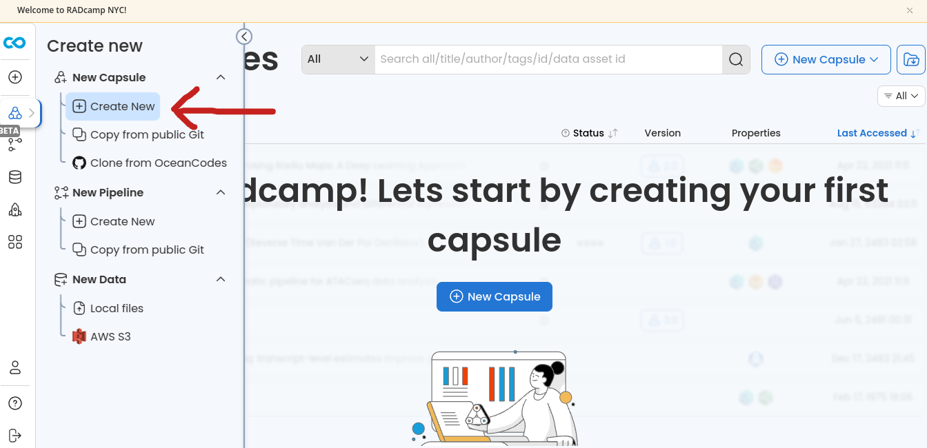
- Log in to the RADCamp CodeOcean instance (https://radcamp.codeocean.com/)
-
On the landing page choose “New Capsule” and then “Create New”
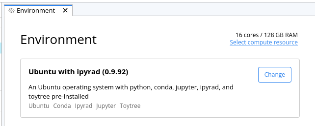
- Select the “Ubuntu with ipyrad (0.9.92)” Environment
-
Choose ‘Select compute resources’ and change it to 16 cores/128GB RAM
-
Now we are going to “launch a cloud workstation” with JupyterLab enabled:
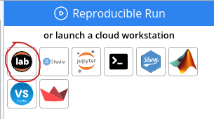
- A bunch of stuff happens with progress bars and moments later you will see
the ‘JupyterLab’ interface, which is our UI to the cloud computers provided by CO.
We will learn more about Jupyter notebooks later in the workshop, but for now
click on “Terminal” in the launcher window.
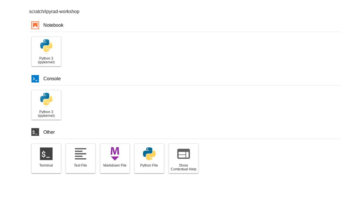
The commands you type in this terminal are not run on your own computer, they are
run on a 16 core virtual machine somewhere out in the ether:
Navigating the command line
Each grey cell in this tutorial indicates a command line interaction.
Lines starting with $ indicate a command that should be executed
in a terminal on the CodeOcean capsule, for example by copying and
pasting the text into your terminal. Elements in code cells surrounded
by angle brackets (e.g.
## Example Code Cell.
## Create an empty file in my home directory called `watdo.txt`
$ touch ~/watdo.txt

## Print "wat" to the screen
$ echo "wat"
wat
Here we’ll use bash commands and command line arguments. If you have trouble remembering the different commands, you can find some very useful commands on this cheat sheet. Take a look at the contents of the folder you’re currently in.
$ ls
There are a bunch of folders. To keep things organized, we will create a new
directory which we’ll be using during this Workshop. Use mkdir. And then
navigate into the new folder, using cd.
$ cd /scratch
$ mkdir ipyrad-workshop
$ cd ipyrad-workshop
- Unix tools: cd, ls, less, cat, nano, grep.
NB: A word about the behavoir of different CO directories.
First view of FASTQ data
Goals of this module:
- View and understand the fastq format
- Understand how the RADseq fastq data is related to the 3RAD molecular protocol? See: “How to add PCR duplicate identifier”
- Be able to locate the restriction enzyme recognition sequence, the i7, and inline barcodes on R1 and R2 files.
For this exercise we will use one sample from an Amaranthus dataset
which is also 3RAD. We will download some of these data, using the command wget.
Make sure that you are in the ipyrad-workshop folder you just created. Since
this is paired end data, you’ll need to grab both R1 and R2 files.
$ wget wget https://github.com/radcamp/radcamp.github.io/raw/master/NYC2023/datafiles/Amaranthus_R1_.fastq.gz
$ wget wget https://github.com/radcamp/radcamp.github.io/raw/master/NYC2023/datafiles/Amaranthus_R2_.fastq.gz
Now, we will use the zcat command to read lines of data from this file and
we will trim this to print only the first 20 lines by piping the output to the
head command. Using a pipe (|) like this passes the output from one command to
another and is a common trick in the command line.
Here we have our first look at a fastq formatted file. Each sequenced read is spread over four lines, one of which contains sequence and another the quality scores stored as ASCII characters. The other two lines are used as headers to store information about the read.
$ zcat Amaranthus_R1_.fastq.gz | head -n 20
@NB551405:60:H7T2GAFXY:1:11101:24090:2248 1:N:0:TATCGGTC+CAACCGGG
TTAGGCAATCGGTTATGAGGTTTACGAACAGGTTAAAGGAGTTGAAACTATATTTGGTAAAACAGGACAAGTGCAAGGGG
+
AAAAAEEEEE/EEEAE/AEEEEEEEEEEEEEEEE/EEEEEEEEEAEEEEEEA/EEE<E/EEAEE<EEEEEEEEEEEE<AE
@NB551405:60:H7T2GAFXY:1:11101:4371:2248 1:N:0:TATCGGTC+GTACCAAA
AACTCGTCATCGGCTACATGTGCTATTATCATTGCCATTTATTCTCCTTGAAGTGCACAAACCAGATTGTCTTGTGCTTA
+
AAA/AAAEEEEEEEEEEEEEEEEEEEEEEEEEEEEEEAEEEEEEEEAE<EEEAEEEAE/EAEAEE/EAEEEEEEEEEEEE
@NB551405:60:H7T2GAFXY:1:11101:6626:2248 1:N:0:AACCTCCT+CAGGTGAA
GGTCTACGTATCGGCCTCCATCCGATTCTGTTGTTGGTACTTTGACTTTCATTGTCACGTTTTAAAACTTTGACCACTAT
+
AAAAAEEEEEEEEEEEEEEE/EEEEEEEEEEEEEEEEEEEEEEEEEEEEEEEEEEEEEEEEEEEEEEEEEEEAEEEEEEE
@NB551405:60:H7T2GAFXY:1:11101:18661:2248 1:N:0:AAGTCGAG+GGCGATAA
GGTCTACGTATCGGGCCTAGATTTCCCTAGTTAACAATGGTGGAATGAAATTGAATTGATTAAGCAGGAGGAAAAGGATG
+
AAAAAEEEEEEEEEEEEEEEEEEEEEEEEEEEEEEEEEEEEEEEEEEEAEEEEEEEEEEEEEEEEEEEEEEEEEEEEEEE
@NB551405:60:H7T2GAFXY:1:11101:18275:2248 1:N:0:CATTCGGT+AACACAGG
TCATGGTCAATCGGTTCATGCTAAACACAATTTCAGAAGTAGCTGTTGAAAGAAGATACATAAAATATAATAGAGATACA
+
/AAA//EAEE/EEEEEEEEE/EEEEEE<EEEEAEEAEEEEEAEEAEEAEEEEEEEEEEEEEAEEEEEAEE<AEEEEEEAE
The first is the name of the read (its location on the plate). The second line contains the sequence data. The third line is unused. And the fourth line is the quality scores for the base calls. The FASTQ wikipedia page has a good figure depicting the logic behind how quality scores are encoded.
The pair of sequences at the end of each header line (TATCGGTC+CAACCGGG) are Illumina’s i7 and i5 read sequences. The libraries you created/will be analyzing used the i7 as the participant identifier and the i5 as the PCR duplicate identifier (unique molecular index). So you should see the same i7 across all reads in your fastq file but different i5 sequences across different reads of the fastq file.
A few activities to work through on your own (or in small groups)
- In this data the restriction enzyme leaves a ATCGG overhang. Can you find this sequence in the raw data?
- Why is the overhang sequence not right at the beginning of the R1 reads? What is that other stuff?
- Use zcat and head to view the first 20 lines of R2. See if you can figure out what the overhang sequence is in R2.
Coffee break (10:30-10:50)
ipyrad history, philosophy, and workflow
Lead: Deren
ipyrad CLI simulated data assembly
Lead: Isaac
Exercise: ipyrad command line assembly with simulated data